
- About Us
- Information
-

The Author ensures that the research has been conducted responsibly and ethically with adherence to all relevant regulations. read more..
- For Authors
- For Reviewer
- Manuscript Guidelines
- Membership
- Publication Ethics
-
- Journals
- Reprints
- e-Books
- Videos
- Policies
- Contact Us
 COVID-19
- Submissions


Full Text
Modern Concepts & Developments in Agronomy
Applications of Aqua crop Model for Improved Field Management Strategies and Climate Change Impact Assessment: A Review
Abadi Berhane* and Demelash Kefale
Department of Plant and Horticultural Sciences, Hawassa University, Ethiopia
*Corresponding author: Abadi Berhane, Hawassa University, School of Plant and Horticultural Sciences, Ethiopia
Submission: May 25, 2018;Published: August 20, 2018

ISSN 2637-7659Volume3 Issue2
Abstract
To quantify, integrate and assess the impacts from weather and climate change/variability on crop growth and productivity, crop models have been used for several years as decision support tools in the world. This paper is reviewed to assess applications of Aqua crop model as a decision support tool for simulating and validating crop management practices and climate change adaptation strategies. This model is devised by the FAO irrigation and drainage team. This model is very important especially, to guide as a decision support tool for dry land areas where soil moisture is very critical to affect crop productivity. It maintains the balance between simplicity, accuracy and robustness. The model has been calibrated and validated to simulate growth and productivity of crops, soil moisture balance, water use efficiency, evapo-transpiration and climate change impact assessment in different climate, management (water, fertilizer, sowing date, spacing etc.) practices around the world, especially in areas where soil moisture stress prevails. Maize, wheat, barley, tee, sorghum, pulse crops such as groundnut, soybean, vegetables (tomato, cabbage) have been tested using this model. The model comprehensively uses stress coefficients (water stress, fertilizer and temperature coefficients) to compute the effect of the factors on crop canopy, dry matter, stomatal closure, flowering, pollination and harvest index build up.
Aqua crop model is calibrated for canopy cover expansion (development), dry matter accumulation and Soil Moisture Content (SMC) in the root zone and initial Harvest Index (HIo) under optimal growth conditions, to simulate the crop canopy development, dry matter and soil moisture content under actual growth conditions. The model is validated for its performance to simulate the crop canopy, dry matter, soil moisture balance grain yield (using normalized water productivity function and dry matter and harvest index). There are different statistical indices used to measure the performance or model goodness of fit such as the Root Mean Square Error (RMSE), normalized-root mean square error, index of agreement (d), model efficiency (E) and coefficient of determination (R2). Hence, application of Aqua crop model as a decision support tool to assess impact of climate change, water management strategies (rain-fed, soil water conservation practices like mulching and bunds), sowing date, plant spacing and fertilizer management strategies under different climatic conditions.
Keywords: Aqua crop; Field management; Crop canopy; Above ground biomass; Soil moisture content; Statistical indices
Introduction
Agriculture is diverse and complex. It is more dependent on weather and climate conditions [1]. These days, climate change becoming a big challenge for the agricultural sector; crop productivity, natural resources, biodiversity and food security; particularly in developing countries due to their low adaptation capacity. Climatic conditions, crop management practices and biotic factors affect crop growth and productivity. However, it is complex to integrate the effect of these processes and analyze the effect on growth and productivity of crop plants. Whereas, crop models have the ability to process and analyze growth and productivity of crops as a function of growth factors such as soil nutrients, soil salinity, drainage, soil moisture, temperature, tillage practices, irrigation methods (furrow irrigation, drip irrigation and sprinkler irrigation), mulching, sowing date, seed rate, rainfall weed management, insect pests and diseases.
Climatic factors are affected by temperature, wind, rain, drought that people feel comfortable or not comfortable in the area because the planning and management are not well. Some of studies show that there is the range of bioclimatic comfort zone which people feel comfortable. Drought evaluation is very important as well as climatic ranges. Drought assessments give people an active scenario in the city to protect the damaging socioeconomic and politic problems. Recent studies with drought stress using remote sensing shows monitoring of drought stress. It is envisaged that both current land uses and future potential future use will be affected by the negative consequences of possible sea-level rise. The morphological structure of low elevations suggests that the effects of elevation can easily proceed to the interior [2-8].
Crop simulation models are now widely used to hypothesize ways to improve agricultural production under seasonal and daily variability of weather [9]. So, modelling has come into application in the agriculture because of several reasons
1. More comprehension about the processes that take place at the Soil-Water-Atmosphere continuum (SWA).
2. Specialists from different fields come to work together.
3. Different and more efficient codes for obtaining the solutions of complex equations were introduced.
4. Amazing development of hardware and supporting software.
5. Large data banks coming from a lot of years of experimental laboratories and field work (mainly at the developed countries).
6. Desire to put together as much SWA processes as possible to get a better comprehension of such a complex system.
As the society become more computerized, there will be more scope for the application crop simulation models to help provide guidance in solving real-world problems related to agricultural sustainability, food security, the use of natural resources and protection of the environment [10]. Modelling of future impacts on complex food security system is still very much a research subject, especially for addressing local impacts in agro-ecological zones at the national level, hence, countries and international communities would greatly benefit from the creation of detailed national and international knowledge and data bases of impacts on the four components of food security [11].
Among the various types of crop models, Aqua crop model maintains a balance between accuracy, simplicity, robustness, and ease of use [12]. The model is aimed at practical end users such as extension specialists, water managers, personnel of irrigation organizations, and economists and policy specialists who use simple models for planning and scenario analysis [13]. It has been applied on a wide range of crops such as forage crops, vegetable, grains, fruits, root and tuber crops [13] on different soils, climatic conditions and management practices in different countries in the world. Information on the different stress coefficients (Ks), conservative and user specific parameters, input and output parameters are not easily accessible to users are not available easily and compiled together with the different management practices and applications. Hence, this paper is reviewed to assess application of Aqua crop model in crop growth simulation models as decision support tool and implications for climate change adaptation, crop productivity and food security; and provide a comprehensive review on the different crop parameters, crop coefficients; calibration and validation procedures for the ease of access to users.
Objectives
The main objective of this paper is to assess application of Aqua Crop model under different soil, climate and management practices with the following specific objectives:
1. To explore the concepts and principles of Aqua Crop model.
2. To assess Aqua crop model applications as on-farm decision support tool under different soil, climate and management practices.
3. To identify suitable climate change adaptation strategies for improved crop productivity and food security.
Crop Growth Simulation Models: Definitions and Concepts
Crop simulation models improve the understanding of crop characteristics of crop growth and development, physiological mechanisms, supporting in applications for data extrapolation and prediction [14]. Crop model, it is a simple representation of a crop growth [15], whereas, a model is a representation of a system with set of equations expressing the behaviour of a system. Models simulate or imitate the behaviour of a crop, its growth and components such as leaves, roots, stems and yield, and other processes in relation to the growth and development of a crop such as soil water processes on a daily basis, climatic and management practices [16]. Crop simulation models integrate the current state of the art scientific knowledge from many different disciplines, including crop physiology, plant breeding agronomy, agro-meteorology, soil physics, soil chemistry, soil fertility, plant pathology, plant entomology, economics and many others. Crop models important in evaluating genetic improvement, for analyzing past genetic improvements from experimental data, and for proposing plant ideo types for larger environments [9] for agroadvisory for weather and diseases impacts.
Crop models represent the real crop growth and development under varying soil and climatic conditions. The changing climatic conditions, dynamic soil factors, genetic and management practices affect the growth and yield of crops. Seasonal and daily variations in weather are major determinants of cropping practices, crop yield, diseases and crop quality. So, crop simulation models have capabilities to predict crop growth response to weather, soils, crop management and genetic factors [9]. Crop simulation models consider the complex interactions between weather, soil properties, crop management factors which influence crop performance; so, crop simulation models are complementary tools in field experiments to develop innovative crop management systems.
Types of crop models
There are many types of crop models, based on the objective, type of crop and model complexity. Generally, crop models can be descriptive models or explanatory models. However, the distinction is not always clear because most process-based models also include empirical relationships, but purely empirical models such as regression models are quite distinct [1]. Generally, crop models can be categorized as descriptive and explanatory models.
Simulation models: These type of models are designed for the purpose of imitating the behaviour of a system at a short time intervals (daily time step) integrating with the daily weather and soil conditions; offering the possibility of specifying management options and investigate a wide range of management practices [16]. These types of models use one or more sets of differential equations, and calculate both the rate and state variables over time (planting until harvest of final product) [17].
Optimizing models: These models have are used for deciding the best option in terms of management inputs for practical operation of the system; deriving solutions, with some optimizing algorithm [16].
Static models: Static model is one that does not contain time as a variable even though crop products of are accumulated over time [17].
Dynamistic models: These models provide predictions for quantities, example: crop yield or rainfall, without any associated probability distribution, variance, or random element. In some cases, dynamistic models may be adequate despite these inherent variations but in some cases they might be unsatisfactory in predicting rainfall [16]. These types of models are used to adjust the response of crops to the climatic factors such as light, heat and water, soil factors such as availability of nutrients and water, presence of toxic elements and physical characteristics of soils, and biological factors like insect pests, diseases and competition with other plants.
Descriptive models: A descriptive model simulates the behaviour of a system in a simple way. In descriptive models experimental data are used to find one or more mathematical equations which are able to describe the behaviour of a system [15]. Empirical models: Empirical model is typically a simplified mathematical model of the system, containing few variables, which are used in crop forecasting; however, they suffer for the lack of realism and generality (ability to be applied in conditions different from those for which they were built). These types of models are based on the direct descriptions of observed data and expressed as regression equations with one or few factors, and are used in yield estimation [17].
Explanatory models: Such models consist of a quantitative description of the mechanism and processes that guide the behavior of a system. Explanatory crop growth models calculate rate variables such as photosynthesis, leaf area expansion, etc.; and state variables (crop biomass, yield, etc.) [15]. These types of models are used in irrigation applications using water balance.
Crop model applications
Crop growth models can be used in research and application (yield predictions, agricultural planning, farm management, climatology and agro-meteorology). Crop growth models have been used to determine the potential growth and establish the biological limits of agricultural production, and predict crop yield, extrapolate and to interpolate crop performances over large regions and to create links with other sciences [15]. Application of crop simulation models can be:
A. Environmental characterization.
B. Optimizing crop management.
C. Pest and diseases management.
D. Impact of climate change.
E. Yield forecasting.
F. Optimal sowing dates.
According to Darko et al. [16] crop model applications can be summarized as,
1. Research understanding: model development ensures the integration of research understanding acquired through discreet disciplinary research and allows the identification of major factors that drive the system and can highlight areas where knowledge is insufficient.
2. Integration of knowledge across disciplines.
3. Improvement of experiment documentation and data organization.
4. Site specific experimentation: crop models can be applied for crop growth, productivity and climate and farm practices using local calibrations.
5. Yield analysis: where a model with a sound physiological background is adopted, it is possible to extrapolate to other environments.
6. Climate change projections: crop production is highly dependent on variation in weather and therefore, any change in global climate will have major effects on crop yields and productivity. Climate analysis for present and future climate projects is very important for present and future climate change adaptation strategies.
7. Scoping best management practices: crop models are being used to identify suitable crop management practices which are environmentally friendly and suitably applied for enhancing crop productivity. Example: determining sowing/ planting date, especially in arid and semi-arid areas where irregular and inadequate rainfall prevails. Optimal fertilizer rates, irrigation methods, soil management practices such as tillage, mulching, and runoff can be simulated using crop models. Soil salinity, drainage and/or infiltration processes can be simulated.
8. Yield forecasting: reasonably precise estimates of crop yield over large areas before the actual harvest are of immense value to researchers and farmers for planning.
9. Models that are based on physiological data are capable of supporting extrapolation to alternative cropping cycles and location, thus permitting the quantification of temporal and spatial variability [16].
Limitations of crop models
Accuracy of crop models in simulating crop growth and productivity, soil processes and climate variability and associated processes vary due to inadequate understanding of natural processes and computer power limitations [14,16]. Crop models output quality depends on the quality of input parameters used. Sampling errors affect the accuracy of observed data, accuracy in climate data also have its own effect of performance of crop models. Observed historical weather data for all modelling applications are important; however, the availability of long-term weather data is limited, sometimes the period of record is too short or few parameters are available and at worst only rainfall, and minimum and maximum temperatures can be found [10], so the performance of the models can be affected. The performance of crop models can be affected by the experience of users [14], experimental data measurement accuracy and sampling methods. The quality of field data as model input affects the quality of model outputs; in crop modelling a proverb ‘Garbage in and garbage out’ makes sense.
Aqua Crop Model: Concepts and Description
Aqua crop model maintains the balance between simplicity, robustness and accuracy, is used by many practitioners such as irrigation and water experts, extension workers, government and NGOs, researchers and others for different on-farm management, irrigation planning, climate change adaptation strategies and soil water balance. It is used to simulate growth and productivity of many herbaceous crops under different water, soil and management conditions [12,13,17,18].
Due to its simplicity, robustness and accuracy, Aqua Crop model has been used to simulate and model growth and yield of crops [13]. It has been evaluated to simulate growth and production of maize [12, 13], tee [19], barley, wheat, rice, sunflower, cotton, potato and hot pepper, cabbage, sugarcane and faba bean under different management, soil and climate conditions.
Canopy cover, rooting depth, dry matter and harvestable yield
In Aqua crop, the crop has five major parameters in response of the governing factors; the crop penology, rooting depth, aerial canopy, biomass production and harvestable yield [12]. Aqua crop runs by first calculating the crop canopy development with time on emergence with the conservative parameters of initial canopy cover per seedling (CCo)=plant density X CCo, canopy growth coefficient (CGC) and maximum canopy cover (CCx) [12]. It simulates green canopy cover instead of leaf area index [18]. However, Aqua crop model simulates plant root system from its effective rooting depth and its water extraction pattern; which effective rooting depth defined as the soil depth where most of the root water uptake is taking place [18]. However, based on their species, crops’ rooting depth can vary; as model input, crop rooting depth is calibrated with the soil profile characteristics and extraction pattern (Figure 1).
figure 1:Physiological processes in Aqua crop model.

This graphical elaboration shows that the dynamic physiological processes as a function of climatic and soil dynamics are carried out. Biomass production as a function of evapo-transpiration is produced. Crop yield is converted from biomass a function of harvest index. In Aqua crop, the canopy is expressed through the fraction of green canopy ground cover (CC); for example for nonstressed conditions, the canopy expansion from emergence to full canopy development follows an exponential growth during the first half of the full development, and follows an exponential decay during the second half; and is computed as in the following equation [13].
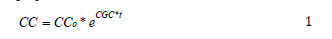
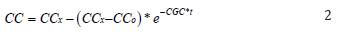
Where CC is the canopy cover at time, CCo is the initial canopy cover, or canopy cover at t=0, CGC is the canopy growth coefficient in fraction per day or per degree day, CCx is the maximum canopy cover, and t is the time in days or degree days.
Maintaining the original concept of a direct link between crop water use and crop yield, the Aqua crop model evolved from the FAO Irrigation and Drainage paper NO. 33 approach, by separating nonproductive soil evaporation (E) from productive crop transpiration (Tr) and estimating biomass directly from actual crop transpiration through a water productivity parameter. The changes lead to the following equation, which is at the core of the Aqua crop growth engine. In this regard, daily biomass is simulated as a function of water productivity normalized for daily transpiration and CO2.
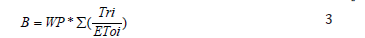
Where, B is the biomass produced cumulatively (kg/m2), Tri and EToi are the daily crop transpiration and reference evapo-transpiration (either mm or m3 per unit surface), with the summation over the time period in which the biomass is produced, and WP is the water productivity parameter (either kg of biomass per m2 and per mm, or kg of biomass per m3 of water transpired). For most crops, only part of the biomass produced is partitioned to the harvested organs to give yield (Y), and the ration of yield to biomass is known as harvest index (HI), hence:
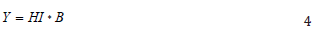
The underlying processes culminating in B and in HI are largely distinct from each other. Therefore, separation of Y into B and HI makes it possible to consider effects of environmental conditions and stress on B and HI separately. Generally, the entire calculation scheme in Aqua crop model is depicted in Figure 2. CC is the simulated canopy cover, CC pot the potential canopy cover, Ks the water stress coefficient, Kcb the crop coefficient, ETo the reference evapo transpiration, WP* the normalized crop water productivity, and HI the harvest index
figure 2:Calculation Scheme of Aqua crop with Indication (dotted arrows) of the processes (a to e) affected by water stress.

Yield response factor
What is yield response factor?: Under water deficit conditions, crop growth and yield is affected. The impact of water stress varies from species to species. In order to quantify the effect of water stress, it is necessary to derive the relationship between relative yield decrease and relative evapo-transpiration deficit is given by the empirically derived yield response factor (Ky).
Yield response factor (Ky) captures the essence of the complex linkages between production and water use by a crop, where many biological, physical and chemical processes are involved. The yield response factor is determined by the empirically by equation [19,20], Crop yield response at different growth stages is computed as
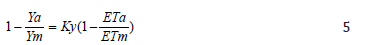
Where, Yx and Ya are the maximum and actual yields, ETx and ETa are the maximum and actual evapo transpiration, and Ky is a yield response factor representing the effect of a reduction in evapo transpiration on yield losses. This equation is called the water production function. According to Steduto et al. [20], the Ky values are crop specific and vary over the growing season according to growth stages with
a. Ky>1: Crop response is very sensitive to water deficit with proportional larger yield reductions when water use is reduced because of stress.
b. Ky< 1: Crop is more tolerant to water deficit, and recovers partially from stress, exhibiting less than proportional reductions in yield with reduced water use.
c. Ky=1: Yield reduction is directly proportional to reduced water use.
Table 1: Seasonal Ky values from FAO Irrigation and Drainage Paper No.33.

Table 2: Soil water stress coefficients and their effect on crop growth.

Crop yield response to water differs from species to species. The different yield response factors (Ky) of different crops are shown in Table 1. Susceptibility to water stress of crops’ varies from species to species and from growth stage to growth stage within a species. The flowering and yield formation stages are sensitive, while stress occurring during ripening stages has limited impact; similarly, the vegetative stage is less affected by water stress, provided that the crop is able to recover from water stress [20]. The Ky values of crops at different growth stages is provided in Table 2.
Yield response factor implications
The yield response to water deficit of different crops is of major importance in production planning. For example, under conditions of limited water supply and with water deficit equally spread over the growing season, the yield decrease for maize (total growing period Ky=1.25) will be greater than for sorghum (Ky=0.9). Consequently, when such crops are grown within the same project areas and maximum production per unit volume of water is being aimed at, maize would have the priority for water supply. When maximum total production for the project areas is being aimed at, and land is not a restricting factor, the available water supply would be directed toward fully meeting the water requirement of maize over a restricted area; for sorghum, the overall production will increase by extending the area under irrigation without fully meeting water requirements provided water deficits do not exceed certain critical values.
Calculation procedures
The calculation procedures for equation 1 to determine actual yield Ya has four steps;
a. Estimate maximum yield (Yx) of an adapted crop variety, as determined by its genetic makeup and climate, assuming agronomic factors example: water, fertilizer, pests and diseases are not limiting.
b. Calculate maximum evapo-transpiration (ETx) according to established methodologies and considering that crop water requirements are fully met.
c. Determine actual crop evapo-transpiration (Eta) under the specific situation, as determined by the available water supply to the crop.
d. Evaluate actual yield (Ya) through the proper selection of the response factor (Ky) for the full growing season or over the different growing stages.
How to calculate maximum yield (Yx)
Maximum yield level of a crop (Yx) is primarily determined by its genetic characteristics and how well the crop is adapted to the prevailing environment. Maximum yield of a crop (Yx) is defined as the harvested yield of a high producing variety, well-adapted to the given growing environment, including the time available to reach maturity, under conditions where, nutrients and pests and diseases do not limit yield.
How to calculate maximum ET
Maximum evapo-transpiration (ETx) refers to conditions when water is adequate for unrestricted growth and development; ETx represents the rate of maximum evapo-transpiration of a healthy crop, grown in large fields under optimum agronomic and irrigation management; hence ETx is computed from the reference evapotranspiration (ETo) and crop coefficient (KC) [20].

figure 3:Linear water production functions for maize subjected to water deficits occurring during the vegetative, flowering, yield formation and ripening periods.

The steeper the slope (i.e. the higher the Ky value), the greater the reduction of yield for a given reduction in ET because of water deficits in the specific period (Figure 3).
Aqua crop model applications for irrigation water management and soil moisture balance
Application of Aqua crop model in irrigation water management: Climate change is an important natural phenomenon which affects crop productivity and food security. Water has always been the main factor limiting crop production in the world where rainfall is insufficient to meet the crop demand [12,20]. In Aqua crop, the water management considers.
1. Rain-fed agriculture with no irrigation.
2. Irrigation: In this parameter, the user defines and selects the type of irrigation applied in the experiment; which might be drip irrigation, sprinkler irrigation, or surface irrigation either by furrow or flood irrigation; the depth of water, and irrigation schedule (the model can automatically generate the irrigation scheduling based on the fixed interval, depth or percentage of soil moisture.
3. In this case, irrigation can be used as supplemental and deficit irrigation.
Under rain-fed conditions efficient use of irrigation water is useful for improved crop productivity and climate change adaption. Hence, Aqua crop model is a water-driven simulation model that requires a relatively low number of parameters and input data to simulate yield response to water of most field and vegetable crops cultivated in the world. It has been used for applications in water management, irrigation scheduling and deficit irrigation applications of many field crops; such as wheat, maize [13], tee [19], barley [19], cotton [18,21] etc.
Aqua crop model is applied to compute crop irrigation water requirement (ETC), simulate crop canopy cover, dry matter accumulation, grain yield, soil drainage and water balance in the root zone, and climate change impact assessment. The model simulates irrigation applications either in the form of deficit irrigation and/or full irrigation applications. Particularly, in arid and semi-arid environments, application of Aqua crop model for applications in deficit or supplementary irrigation has paramount importance in improving crop water productivity and irrigation water use efficiency. The analysis of deficit irrigation studies allowed for majority of crops, the development of crop response functions when water deficits occur at different crop stages [20].
Aqua crop describes water stress effects by stress coeffiencets (Ks); which above the upper threshold root zone depletion, water stress is non-existent (ks is 1), and the process is not affected; however, soil water stress starts to affect a particular process, when the stored soil water in the root zone drops below the upper threshold level, and below the lower threshold level, the effect is maximum (Ks is 0) and the process is completely halted. The four coefficients are leaf growth, stomatal conductance, canopy senescence, and pollination failure [13].
Application of Aqua crop model for simulating soil moisture balance
Aqua crop is configured as a dispersed system of a variable depth allowing up to 5 layers of different texture composition along the profile, including all the classical textural classes present in the USDA triangle [12]. Aqua crop performs a daily water balance that includes all the incoming and outgoing water fluxes (infiltration, runoff, deep percolation, evaporation and transpiration) and changes in water content [13]. A daily step soil water balance keeps track of the incoming and outgoing water fluxes at the boundaries of the root zone and of the stored soil water retained in the root zone [13]. So, soil water balance is critical in the daily physical and physiological processes of crops.
The unique feature of water balance in Aqua crop model is the separation of soil evaporation (Es) from the crop transpiration (Tc); in the simulation of Es, Aqua crop includes the effects of mulching, withered canopy cover, partial wetting by localized irrigation, and the shading of the ground by the canopy [13]. So, the soil moisture balance is calculated based on the equation.

Where, ETC is crop water requirement, P is precipitation (usually rainfall), I is irrigation, R is runoff, D is drainage, S is change in soil moisture (can be +ve or –ve).
Aqua crop model describes water stress effects on crop physiological processes by stress coefficients (Ks); above the upper threshold root zone depletion, water stress is non-existent (Ks is 1) and the process is not affected; however, soil water stress starts to affect a particular process, when the stored soil water in the root zone drops below the upper threshold level, and below the lower threshold level, the effect is maximum (ks is 0) and the process is completely halted [12] and the effects of soil water stress on different processes are shown in Table 3. Studies on calibration and evaluation of Aqua crop model on different crops and soil types indicate that Aqua crop model has the capacity to simulate the soil moisture content and daily soil water dynamics [13,21].
Table 3: Soil fertility stress coefficients and their effect on crop growth.

Application of Aqua Crop Model in Soil Fertility and Salinity Management
Soil fertility management
Soil fertility is an important factor determining crop growth and productivity. Aqua crop model does not simulate nutrient cycles and balances; it adjusts the fertility effects with a set of soil fertility stress coefficients in for four important components of productivity; the canopy growth coefficient (CGC), maximum canopy cover (CCx), canopy decline (CDC) and water productivity [22]. Soil fertility stress indicator varies from 0% at which soil fertility is non-limiting, to 100% when soil fertility stress is so sever and crop production is no longer possible, with soil fertility coefficients (Ks) ranging from 1 (no soil fertility stress) to 0 (full soil fertility stress) [12]. Canopy development and biomass production might be affected by soil fertility stress. The stress coefficients considered by Aqua crop and their effects on crop growth are described in Table 4.
Table 4: Soil salinity stress coefficients.

Salt balance and soil salinity management
Soil fertility stress is indicated by the average electrical conductivity of saturation soil-paste from the root zone [20]. In Aqua crop the incoming and outgoing salt fluxes can be simulated. Salts enter and leached out of the soil with downward water movement; and enter from upward transport of saline water from a shallow water table. The upper and lower salinity stress coefficients (Ks) are 0 and 1 respectively. At the lower threshold soil salinity (ECe) the salinity stress starts to affect crop growth, and the Ks values is less than 1; however, the upper threshold soil salinity threshold (Ks) starts and becomes sever affecting crop growth and development, and the growth becomes to cease and reaches zero. The effect of soil salinity stress coefficients on different crop growth parameters is shown as below Table 4.
Aqua crop model applications for climate change adaptation and mitigation strategies
Climate change predictions indicate a warmer world within the next 50 years, however, impact of rising temperatures on rainfall distribution patterns in the semi-arid tropics (SAT) of Africa and Asia remains far less certain. Impact of climate change has been assessed for the present and future. It has been indicated that there will be climate change variability in the future (2030 and 2050) which will have a substantial impact on crop growth and productivity [19]. Studies on climate change projection in at different sites in Ethiopia indicate that there is an increase in maximum and minimum temperature in the future. Increasing CO2 concentration at the different scenarios will affect crop productivity from mid to the end of the 21st century. The temporal and spatial rainfall variability will affect crop growth and productivity. So, adjusting sowing and supplementary irrigation has been found important adaptation options.
Statistical indices used to measure aqua crop model efficiency
Aqua crop model simulates observed crop and soil moisture parameters based on the calibrated parameters and inputs. However, the simulated parameters such as soil moisture content, dry matter, crop canopy cover, transpiration, runoff and drainage, can be efficiently or accurately simulated. But the model efficiency has to be measured based on statistical indices to how much the simulated data are close to the observed data.
Root mean square error (RMSE): RMSE represents a measure of the overall, or mean deviation between observed and simulated values, which is an indicator of the uncertainty of the model; the closer the value is to zero, the better the model simulation performance [13]. The unit of this RMSE is the same with the unit of the measured or observed values.
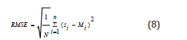
Where, Si is the simulated value, Mi is the measured value, and n is the number of observations. RMSE takes the unit of the observed and simulated values.
Coefficient of efficiency (E): Coefficient of efficiency is (Nash and Sutcliffie, 1970) also another statistical index used to how much the model is efficient in simulating the observed data.
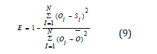
The coefficient of efficiency (E) expresses how much the overall deviation between the observed and simulated values departs from the mean value (Om); this index compared to the RMSE, it is able to capture how well the model performs over the entire simulation span [12]. E is unit less with values assumed to range from -∞ to+1. Si and Oi are the simulated and observed values, respectively; Om is the mean of the observed values. N is the number of observations. The smaller the deviation from (Oi-Om), the higher the efficiency of the model.
Index of agreement (d): Index of agreement [23] is another statistical index used to measure the Aqua crop model efficiency. The value of d varies from -∞ to +1. The closer the value to +1 indicates the better the model efficiency is.
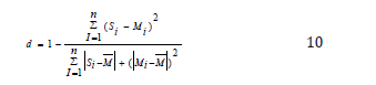
Where M ̅ is the mean of the n measured values, Si and Mi are the simulated and measured values.
Normalized root mean square error (N-RMSE): The new versions of Aqua Crop model (version 5 and 6) contains the normalized RMSE which observed and simulated parameters are compared. The smaller the value, the better the agreement will be [24,25].
Coefficient of determination (R2): This statistical index is also another measurement of model goodness of fit. In Aqua crop, in addition to the index of agreement (d), RMSE and N-RMSE, this R2 is an indicator of the efficiency of the model in comparing the measured values with the predicted values. It explains the amount of the variance explained by the model in comparison to the observed values. The value of the coefficient of determination (R2) ranges from 0 to 1; the better value closer to 1, the better the efficiency of the model will be.
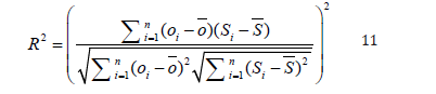
Where, Oi and Si are the observed and simulated values, O ̅, S ̅ are mean of the observed and simulated values.
Conclusion and Recommendation
Crop models have been used widely for several years to hypothesize ways to improve agricultural productivity under varying climatic and soil conditions, and management practices. Crop models are being applied to assess effect of climate change on crop growth and productivity, to simulate soil water balance (outgoing and ingoing water flux), to simulate canopy cover (LAI), Dry Matter accumulation (dm) and crop yield. Depending on the objectives, crop models are used as decision support tools to on-farm management practices (example: irrigation, soil water conservation, runoff) and crop genetics; and to assess water and nutrient stress at various growth stages. Crop models are used to determine, crop Water Use Efficiency (WUE) and/water productivity, irrigation scheduling and operations, planting/ sowing date; and food security implications for policy making. Spatial and temporal rainfall and temperature variability effects can be assessed using crop modelling [26].
In the field of crop modelling, there is a need for integrated research in a way that multidisciplinary activities and professions participate (computer engineers, agronomists, economists, breeders, soil scientists, climate, etc.) for comprehensive and broad range research outputs are produced. So, crop modelling has the potential to simulate soil moisture balance, crop growth and productivity under optimal and sub-optimal water and fertilizer levels, hence farmers can benefit from these research outputs, and thereby enhance their productivity and ultimately their food security [27].
Aqua crop, DSSAT, APSIM and Wofost (yield gap) models have been applied in different areas to study the effect of soil moisture stress, deficit irrigation (Supplemental irrigation), nutrient stress (in particular to nitrogen), sowing date and effect of climate change on crop growth and productivity in Ethiopia. Aqua crop model maintains the balance between simplicity, robustness and accuracy in simulating crop growth and management strategies under different climatic, soil and management. It simulates crop canopy cover, biomass development, soil moisture balance using different stress coefficients (stomatal closure, canopy expansion, pollination, flowering etc.) [28].
Performance of Aqua crop model in simulating crop canopy, dry matter, soil moisture balance, grain yield, evapo-transpiration, water use efficiency and runoff, is measured statistical indices such as root mean square error, normalized root mean square error, index of agreement, and model efficiency. Crop models (Aqua crop model in this discussion) can be applied to assess the negative effects of climate change under present and future climate [29,30]. Therefore, government, policy makers and other stakeholders in agricultural researches should give emphasis in modern researches, capacity building (training, workshops, experience sharing), financial support, infrastructures (laboratories, tools and equipments). Universities, research centres, NGOs and other stakeholders are less responsive in creating modern researches towards the end of the 21st century; and inter or intra-organizational communication or relationships are poor. So, integrated and wider scope agricultural researches are demanding to achieve food security and improve livelihood of subsistence farmers in Ethiopia.
References
- Müller C, Elliot J (2015) The global gridded crop model intercomparison: Approaches and caveats for modelling climate, Insights change impacts on agriculture at the global scale. In: Elbehri A (Ed.), Climate change and food systems global assessments and implications for food security and trade. FAO, Rome, Italy.
- Cetin M (2015a) Determining the bioclimatic comfort in Kastamonu City. Environmental Monitoring and Assessment 187(10): 640.
- Cetin M (2015b) Using GIS analysis to assess urban green space in terms of accessibility: Case study in Kutahya. International Journal of Sustainable Development & World Ecology 22(5): 420-424.
- Cetin M, Sevik H (2016) Evaluating the recreation potential of Ilgaz mountain national park in Turkey. Environmental Monitoring and Assessment 188(1): 52.
- Cetin M (2016) Sustainability of urban coastal area management: A case study on Cide. Journal of Sustainable Forestry 35 (7): 527–541.
- Cetin M, Adiguzel F, Kaya O, Sahap A (2018) Mapping of bioclimatic comfort for potential planning using GIS in Aydin. Environment Development and Sustainability 20(1): 361-375.
- Cetin M, Zeren I, Sevik H, Cakir C, Akpinar H (2018) A study on the determination of the natural parks sustainable tourism potential. Environ Monit Assess 190(3): 167.
- Yucedag C, Kaya LG, Cetin M (2018) Identifying and assessing environmental awareness of hotel and restaurant employees attitudes in the Amasra District of Bartin. Environmental Monitoring and Assessment 190: 60.
- Jones JW, Hoogenboom G, Porter CH, Boote KJ, Batchelor W, et al. (2003) The DSSAT cropping system model. European Journal of Agronomy 18(3-4): 235-265.
- Hoogenboom G (2000) Contribution of agro meteorology to the simulation of crop production and its applications. Agricultural and Forest Meteorology 103(1-2): 137-157.
- (2008) Climate change adaptation and mitigation in the food and agriculture sector. FAO, Rome, Italy.
- Hsiao TC, Heng L, Steduto P, Rojas Lara B, Raes D, et al. (2009) Aqua crop the FAO crop model to simulate yield response to water: III, parameterization and testing for maize. Agronomy Journal Abstract 101(3): 448-459.
- Heng LK, Hhsiao T, Evett S, Howell T, Steduto P (2009) Validating of the FAO aqua crop model for irrigated and water deficient field maize. Agronomy Journal 101(3): 488-498.
- Rauff KO, Bello R (2015) A review of crop growth simulation models as tools for agricultural meteorology. Agricultural Sciences 6(9): 1098- 1105.
- Miglietta F, Bindi M (1993) Crop simulation models for research, farm management and agro-meteorology. Advances in Remote Sensing 2(2): 148-157.
- Darko OP, Yeboah S, Addy S, Amponsah S, Danquah EO (2013) Crop modelling: A tool for agricultural research-a review. Journal of Agricultural Research and Development 2(1): 1-6.
- Murthy VR (2002) Basic principles of agricultural meteorology. Book Syndicate Publishers, India.
- Villa GM, Fereres E, Mateos L, Orgaz F, Steduto P (2009) Deficit irrigation optimization of cotton with aqua crop. Agronomy Journal 101(3): 477- 487.
- Araya A, Kisekka I, Girma A, Hadgu KM, Tegebu, et al. (2016) The challenges and opportunities for wheat production under future climate in northern Ethiopia. Journal of Agricultural Science 155(3): 379-393.
- Vanuyntrecht E, Raes D, Steduto P, Hsiao TC, Fereres E, Heng LK, et al. (2014) Aqua crop: FAO’S crop water productivity and yield response model. Environmental Modelling and Software 62: 351-360.
- Farahani H, Izzi G, Oweis TY (2009) Parameterization and evaluation of the aqua crop model for full and deficit irrigated cotton. Agronomy Journal 101(3): 469-476.
- (2012) Climate change adaptation and mitigation: Challenges and opportunities in the food sector. FAO, Rome, Italy.
- Willmott CJ (1982) Some comments on the evaluation of model performance. Bulletin of American Meteorological Society 63(11): 1309-1313.
- Alemayehu YA, Steyn JM, Annandale JG (2009) FAO-type crop factor determination for irrigation scheduling of hot pepper (capsicum annuum l) cultivars. South African Journal of Plant Soil 26(3): 186-194.
- Conway D, Schipper El (2011) Adaptation to climate change in Africa: Challenges and opportunities identified from Ethiopia. Global Environmental Change 21(1): 227-237.
- (2007) Climate change 2007: Synthesis Report. IPCC, Geneva, Switzerland, pp. 104.
- (2014) Climate change: Synthesis report. Fifth Assessment Synthesis Report. IPCC, Switzerland, pp. 151.
- Keating BA, Carberry PS, Hammer GL, Probert PL, Robertson MJ, et al. (2003) An overview of APSIM, a model desined for farming systems. European Journal of Agronomy 18(3-4): 267-288.
- Nash JE, Sutcliffe JV (1970) River flow forecasting through conceptual models part- I: A discussion of principles. Journal of Hydrology 10(3): 282-290.
- (2007) Climate change National Adaptation Program of Action (NAPA) of Ethiopia. NMA, Addis Ababa, Ethiopia.
© 2018 Abadi Berhane. This is an open access article distributed under the terms of the Creative Commons Attribution License , which permits unrestricted use, distribution, and build upon your work non-commercially.
Editor In Chief


.jpg)


Signup for Newsletter

Quick Links
 Editorial Board Registrations
 Submit your Article
 Refer a Friend
 Advertise With Us
Our Recent Edition

.jpg)


Top Editors


.jpg)


.bmp)
.jpg)
.png)
.jpg)


.jpg)


.png)

.png)


.png)


Financial Support

Sponsors

Latest e-Books

Latest Video

 a Creative Commons Attribution 4.0 International License. Based on a work at www.crimsonpublishers.com.
Best viewed in
a Creative Commons Attribution 4.0 International License. Based on a work at www.crimsonpublishers.com.
Best viewed in