Timeless, Generational Mathematical Model of the Influence of Age Structure on the Change in the Numerical Composition of living Systems

Typically, a mathematical prediction requires an author’s hypothesis about the future, explaining the mathematical result based on clear physical assumptions. In the developed accepted forecasts of the world population, groups of methods are used that involve certain assumptions [1-6]. So, extrapolation methods are performed under the assumption of the invariance of the absolute population growth or growth rate. Analytical methods are since functions are selected based on past demographic dynamics that describe it most closely [7-14]. The component method (age shifting) is based on the use of the demographic balance equation and allows one to obtain not only the total population, but also its distribution by sex and age [15,16]. However, to use the equation of demographic balance, knowledge of the differential rates of birth and death is required.

When using existing mathematical models of demographic dynamics, difficulties also arise in describing the real non-monotony and “jumps” of the dynamic temporal process of population changes. These features of real dynamics are determined by possible specific historically determined interactions of populations with each other, their psychological and biological responses to the effects of various environmental factors of anthropogenic and natural nature [8,17]. Ultimately, they can lead to fundamental deviations from “fate” predicted by evolutionary mathematical models that predict stabilization and sustainable development in optimistic scenarios. Therefore, based on inevitable assumptions and mathematical difficulties in describing and forecasting the population, it is important to have a fundamentally new additional method for assessing the nature of the dynamics of the population, independent of time and influence factors and increasing the degree of reliability of the result.

The dynamics of the population, including a population explosion or stabilization, is determined in any region of residence by the age structure of the population. Typical options for changing the population will be calculated on the basis of the following procedure.

The total number of people born in (K +1) generations can be written in arithmetic progression

Here is the number of people of the initial (zero) generation ( K = 0 ); - the number of children (generation); f - the proportion of couples from each generation dying before the appearance of the immediately following generation; k (small)- generation number; K (large)-the final generation (for example, if great-grandchildren, then K = 3 ).

We confine ourselves to four generations, i.e., k = 0, 1, 2, 3. In this case we get

Suppose that when great-grandchildren are born, then there is no longer a fraction of

the great-grandfathers and the proportion of grandfathers. Then, the number of dead individuals (3) 0, 1 ( , , ) d N g f F F will be determined by the expression

The number of individuals remaining alive will be equal

The relationship we are interested in

defined by the expression

We require that r=1. Then from (6) we obtain:

Consider examples of population stabilization that correspond to the “old” population. Let us accept the following conditions most common in recent years for Russia and some other countries. The average life expectancy of men is approximately 60 years, women- approximately 70 years, “great-grandfathers” (0-th generation) do not live to see the birth of great-grandchildren (F0=1), and the first generation (grandfathers and grandmothers) already have 50% of grandchildren’s birth die (F1=0.5). Suppose also that all parents remain alive (f=0). Then, for population reproduction, it is necessary to have an average of 1.5 children for each couple (male and female) (Figure 1).

Figure 1: Dependence of the minimum permissible birth rate , ensuring the reproduction of people, on the share of “grandfathers” (generation ) who did not live to see their grandchildren (generation ): F0: (1)-1, (2)-0.8, (3)- 0.6, (4)-0.5; ( )-f=0, (---)-f=0.1, (--)-f=0.2.

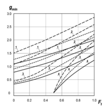
Consider examples of population stabilization that correspond to the "old" population. Let us accept the following conditions most common in recent years for Russia and some other countries. The average life expectancy of men is approximately 60 years, women-approximately 70 years, "great-grandfathers" (0-th generation) do not live to see the birth of great-grandchildren (F₀=1), and the first generation (grandfathers and grandmothers) already have 50% of grandchildren’s birth die (F₁=0.5). Suppose also that all parents remain alive (f=0). Then, for population reproduction, it is necessary to have an average of 1.5 children for each couple (male and female) (Figure 1).

With an older population, if the entire 1st generation does not die by the time of the birth of their grandchildren (F₁=0), it is enough to have 1.1 children on average for each pair. In the case of population rejuvenation, when the 0th and 1st generations die before the birth of great-grandchildren and grandchildren (F₀=1, F₁=1), for reproduction it is necessary to have an average of 2 children for each pair. Even when all the 0-th generation (“great-grandfathers”) die before the birth of the great-grandchildren (F₀=1), the 1^st generation (“grandfathers”) die 40% before the birth of the their grandchildren, and 20% of the 2^nd generation (parents) die before the birth of their children (f=0.2), then for the reproduction of the population (r= ) it is also necessary to have 2 children (g=2).

A population explosion can develop with a young population. For example, if under the previous conditions there will be 3 children in a family, then the population over 4 generations will increase by 2 times (Figure 2). The average number of children per each living heterosexual couple is a criterion for the survival of the population in any region of the world.

Figure 2: The ratio r of the number of living people at the moment of the appearance of great-grandchildren (generation) to the number of people who died by this time, depending on the birth rate: F0=1; F1: (1)-0,(2)-0.4; ( )-f = 0, (- - -)-f=0.2.

In the generational mathematical model proposed above, the analysis of the dynamics of the number of individuals does not require knowledge of their lifetime. Therefore, it is applicable for any biological system that has the property of reproduction. The age structure of a specific totality of individuals is the basis of the model. It can be used, in particular, to assess the nature of changes in the human population in real time and increase the reliability of demographic forecasts, regardless of the time and influence factors.

1. Contemporary Demographic Policy (2007) Russia and foreign experience, analytical bulletin of the federation council of the federal assembly of the Russian federation. No. 25, (in Russian).
2. https://www.cia.gov/libarary/ publications/the-world-factbook/geos/us.html
3. UN population division world population prospects.
4. USA quick facts from the US census bureau.
5. (2015) United nations, department of economic and social affairs, population division.
6. (2015) World population prospects. The 2015 Revision, DVD Edition. File POP/8-1.
7. Anikin AV, Malthusianism (1975) Youth of science: Life and ideas of thinkers-economists before Marx. In: (2^nd edn), Politizdat, Moscow, Russia, pp. 266-274.
8. Viktorov AA, Kholodnov VA (2020) Analysis and forecast based on the kinetic equation for changing the numerical composition of living systems. Gerontology & Geriatric Studies 5(5): 542-548.
9. Kapitsa S (1999) Model of earth's population growth and economic progress of mankind. Economic issues, No. 12.
10. Kapitsa S (1999) How many people lived, lives and will live on the Earth. Nauka, Moscow, Russia.
11. Foerester H, Mora P, Amiot L (1960) Doomsday: Friday, 13 November, A.D. 2026. At this date human population will approach infinity if it grows as it has grown in the last two millennia, Science 132: 1291-1295.
12. Hoerner S (1975) Population explosion and interstellar expansion. Journal of the British Interplanetary Society 28: 691-712.
13. Кrеmеr M (1993) Population growth and technological change: One Million B.C. to 1990. The Quarterly Journal of Economics, 108: 681-716.
14. Verhulst PF (1845) Recherches Mathématiques sur La Loi D’Accroissement de la Population. Nouveaux Mémoires de l’Académie Royale des Sciences et Belles-Lettres de Bruxelles, 18, Art-1, pp. 1-45.
15. Orlov YN (2015) Methods of mathematical demography: state-of-the-art, problems, exact results. Keldysh Institute of Applied Mathematics RAS, MIPT, sector of kinetic equations, department of higher mathematics, KIT, Kotovsk, Russia.
16. Staroverov OV (1997) The basics of mathematical demography. Nauka, Moscow, Russia.
17. Selye G (1982) Stress without distress. In: (1^st edn), Progress Publisher, Moscow, Russia.