
- About Us
- Information
-

The Author ensures that the research has been conducted responsibly and ethically with adherence to all relevant regulations. read more..
- For Authors
- For Reviewer
- Manuscript Guidelines
- Membership
- Publication Ethics
-
- Journals
- Reprints
- e-Books
- Videos
- Policies
- Contact Us
 COVID-19
- Submissions


Full Text
Evolutions in Mechanical Engineering
On Acoustic Properties of Duct Termination Exhausting Hot Flow by Utilizing FEM Simulation
Hans R1* and Jüri L2
1Associate Professor, Tallinn University of Technology (TalTech), Estonia
2Professor, Tallinn University of Technology (TalTech), Estonia
*Corresponding author:Hans R, Associate Professor, Department of Mechanical and Industrial Engineering, Tallinn University of Technology (TalTech), Ehitajate tee 5, Tallinn, 19086, Estonia
Submission: January 11, 2020;Published: April 16, 2021

ISSN 2640-9690 Volume3 Issue3
Abstract
Determination of the acoustical properties for hot flow duct openings is a classical problem in acoustics. The importance of this issue usually becomes apparent when noise radiation from engine exhaust systems or burner chimneys is considered. In the paper a Finite Element Method (FEM) simulation has been applied to investigate the effects of high temperature media on the sound propagation through open duct termination. This paper is an extension for the recent experimental work performed by paper authors on acoustical properties of duct terminations exhausting hot gas. In order to simulate the experimental conditions, commercial FEM software COMSOL has been used. The acoustic pressure reflection coefficient of the duct termination is calculated from the complex pressure values simulated at the location of two microphones in the test-duct model. Two geometrically different simulated configurations for the jet, based on experimental observations, are studied. The numerical results obtained from simulations are compared to the experimental and theoretical ones and good agreement between the data is observed.
Introduction
The acoustical behavior of a circular duct termination exhausting flow has been investigated by the authors of this paper both experimentally [1-3] and by implementing Munt’s theoretical model [4]. The objective of the present study was to compose a FEM model that can be applied to simulate the above-mentioned experimental procedure. Since considerably few attempts to utilize FEM for prediction of acoustical performance of flow duct elements was found from literature the intention was well motivated. The numerical model was developed to test the ability to implement a simple FEM model for determination of the passive acoustic properties of flow duct elements in low Mach number and low Helmholtz number conditions. Additionally, to the intention to verify the experimentally and theoretically obtained results, the model was intended for successive development to perform analysis on various duct termination geometries and flow conditions. The experiments for the acoustical pressure reflection described in [1] were carried out using a thin-walled steel duct with a circular cross-section area. The duct was mounted vertically in a relatively large room and the hot air flow through the test section was generated by two electrical blowers and surface heating elements. The reflection coefficient was determined by using the two-microphone approach [5,6]. A simplified layout of the experimental set-up used for the experiments is presented in Figure 1. In order to characterize the temperature distribution and the geometry of the exhausting jet, a series of flow visualization experiments together with temperature mapping around the opening were carried out (see Section 3). This information was primarily important for the composition of the FEM models.
Figure 1:A simplified layout of the setup used for experiments [1,2] and followed by the FEM models.

Following the experimental conditions and corresponding test duct geometry, a three-dimensional FEM model was created using a commercial software COMSOL 3.3. In order to analyze the influence of variations in the jet geometry on the acoustical properties, two different models – one with cylindrical and another with conical jet were tested. An overview of the modelling procedure is provided in Section 3.2. Two microphone method (see Section 4.1.1) was followed to determine the acoustical pressure reflection coefficient by using the complex pressures directly obtained from FEM simulations (see Section 4.1.2). The FEM simulation procedure was run sequentially at eleven evenly separated discrete frequencies points to cover the range from 10 to 3000Hz. Three average jet temperatures (100, 300 and 500°C) were selected to perform the simulations. For a substantially simpler numerical process and less demanding computational effort the flow effects were neglected in the models, following the experiments [1] where the flow Mach number was kept low (M<0.01). In Section 5 the modelling results for the temperature conditions analysis are presented. The experimental results for the same jet temperatures are included for comparison.
Temperature Mapping and Flow Visualization
The flow visualization was performed by using an infra-red (IR) imaging camera (Flir systems, Thermacam S65). In order to capture the hot jet with reasonable clarity, smoke particles were generated in the flow by spraying oil into the hot test section. Despite of a roughly cylindrical shape of the jet observed Figure 2 a tendency to conical shape can still be noticed at the distance about 0.25m from the opening. It can be mentioned here that the considerable density difference between the jet and the surrounding media (about 2 times for a 300 °C jet exhausting into a room temperature air) normally leads to a phenomenon known as accelerated flow. In such a flow condition even a decrease in the jet diameter can be expected in the region after passing the duct lips. The latter seems to be in agreement with the IR images, Figure 2, around 0.2m downstream from the pipe opening. Additionally, to the IRimaging, a temperature mapping using a dual K-type thermometer (TES1312) were carried out in the region around the duct outlet. The temperature readings were taken at the crossing points of the grid Figures 2 & 3 that extended up to 1m from the termination along the duct central axis and up to 0.4m in radial direction. Assuming symmetry, the readings were taken only on one side of the plane. An example of the mapped temperature data for 300 °C and 2.5m/s airflow is shown in Figure 3. It can be seen that influence of the hot jet on surrounding room temperature (25 °C) did not extend further than around 0.2m (about 4 duct diameters) in the radial direction from the duct central axis.
Figure 2: An example of IR camera image captured during the flow visualization experiments; Jet temperature at the exit: t=300 °C, flow velocity: v=2.5m/s; The 0.1 by 0.1m grid represents the locations of the temperature readings.

Figure 3: Temperature distribution near the test duct termination; t = 300 ºC, v=2.5m/s. Along the duct central axis (circles), 0.1m from central axis (triangles), 0.2m from central axis (stars), 0.3m from central axis (x-s), 0.4m from central axis (squares).

Simulation Procedure
Determination of the acoustic pressure reflection coefficient
Assuming linear and passive termination in the positive x-direction Figure 4 and concerning only of a plane wave state, the reflection coefficient can be determined in this direction as:
Figure 4: Model configuration following the two-microphone approach.

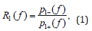
where p1− , p1+ is the acoustic pressure field generated by the simulation model at the microphone 1 cross-section (defined as a reference cross-section). Following the two-microphone method [5-7], the incident and reflected pressure wave amplitudes p1+(f) and p1−(f) can be calculated at the reference cross-section by using two microphone positions Figures 1 & 4 as follows:
where p is the acoustic pressure, f is the frequency, k = 2πf / c is the wave number, c is the speed of sound, s represents the microphone separation, - and + denote the pressure waves propagating in neg. and pos. direction relative to the x-axis, k− = k /( 1− M) , k+ = k /( 1+ M) and M is the Mach number. Indexes 1 and 2 refer to the microphone positions. In the current paper the complex acoustic pressure values p1(f) and p2(f) are the FEM simulation results which are used for the reflection coefficient calculation as the input parameters. By combining the Eqs. (2) and (3), the expressions for p1+(f) and p1−(f) will be obtained as follows:
In order to determine the reflection coefficient at the duct termination cross-section, it is necessary to move R1 to this location. This can be done by using the equation:
where l is the distance from the reference cross-section to the duct termination.
The simulation model
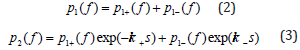
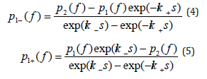
Commercial finite element method software (COMSOL Multiphysics) [8] was used to create the simulation model for determination of the acoustic pressure reflection at the opening. A similar FEM model of the pipe opening was composed by Kierkegaard [9] for investigation of the acoustic radiation from a chimney exhausting hot exhaust gas. The model was found to perform adequately to study the radiation phenomena. In this paper the finite element model was focused on the simulation of the complex acoustic pressures ( ) 1 p f and ( ) 2 p f at the virtual pressure transducer cross-sections inside the flow duct. Two geometrically different jet models were tested in this study. Firstly, a cylindrical model of the hot jet was composed as shown in Figure 5, followed by a second model with conical jet geometry (Figure 6). The angle of expansion of the conical jet was chosen 16°. Such a relatively large angle was selected in order to investigate the effect of jet geometry on the results in the artificially exaggerated form. For both 3-D models created the dimensions of the test-duct model followed the ones of the experimental pipe [1]. The duct walls (with 2mm thickness) were defined as acoustically hard, which means that the gradient of the sound pressure field in the normal direction of the duct was always zero. In order to keep the calculation time reasonable, the space surrounding the duct termination model Figure 5 was reduced to a prism (height h=1.3m, and the base area A=1 by 1m).
Figure 5: An image of the FEM model with cylindrical jet geometry. The duct termination is modelled inside the surrounding volume.

Properties of air at room temperature (25 °C) and the normal pressure were defined inside the surrounding volume. A radiation condition was determined to represent the boundary conditions of the prism surface areas. This boundary condition behaves like a surface where all the incident waves are transmitted outside of the prism and not being reflected back to the duct, as expected in the experimental case. The duct termination was located at the height of 0.3m from the bottom surface along the vertical central axis of prism. Uniform and homogeneous acoustical conditions were defined for the jet in each simulated temperature case. The hot jet was modelled to fill the test duct internal volume completely and to extend out of the termination up to the limiting surface of the surrounding prism (1m from the termination) either following the cylindrical shape or conically (Figures 5 & 6). A continuity condition was set to represent the boundary conditions at the shear surface between the jet and the surrounding media. At the inlet plane of the duct a fluctuating sound pressure providing the acoustic excitation was imposed with amplitude of 20Pa. It should be noted here that assuming a linear model this value can be scaled to any other number without affecting the results. The simulations were repeated for eleven excitation frequencies to cover the range from 10 to 3000Hz. After the solution was achieved, it was necessary to post-process the results in order to record the acoustic pressures p1(f) and p2(f). These values were found by evaluating the complex pressures at the axial coordinates along the duct inner surface representing the locations of the virtual pressure transducer. The simulated pressure values were then inserted into the calculation module to determine the acoustic pressure reflection coefficient, following the procedure described in Section 3.1. This process was sequentially repeated for every excitation frequency selected.
Figure 6: An image of the FEM model with conical jet geometry.

Results
The numerically determined magnitude and phase of the reflection coefficients for all the modelled jet temperatures are presented in Figures 7-12. The corresponding results obtained experimentally are included in comparison. The agreement between the results is good for all the temperatures. The figures show that the two geometrically different jet models produce relatively similar results. However, it can be noticed that in some cases the results from the cylindrical model are in marginally better correlation with the measured ones. The reason for this can be related to more realistic jet geometry of the cylindrical model, regarding the flow visualization results. In Figure 13 the reflection coefficient magnitude is presented for 100 °C and 500 °C jet temperatures. In this figure the results obtained by implementing Munt’s theoretical model [4] are additionally included in comparison. As can be observed the correlation of the results is good and the discrepancy typically remains within 5%.
Figure 7:The magnitude of the reflection coefficient for duct open termination; t = 100 ºC, Experiments (circles), FEM - conical model (diamonds), FEM - cylindrical model (stars).

Figure 8:The phase of the reflection coefficient for duct open termination; t = 100 ºC, Experiments (circles), FEM - conical model (diamonds), FEM - cylindrical model (stars).

Figure 9:The magnitude of the reflection coefficient for duct open termination; t = 300 ºC, Experiments (circles), FEM - conical model (diamonds), FEM - cylindrical model (stars).

Figure 10: The phase of the reflection coefficient for duct open termination; t = 300 ºC, Experiments (circles), FEM - conical model (diamonds), FEM - cylindrical model (stars).

Figure 11: The magnitude of the reflection coefficient for duct open termination; t = 500 ºC, Experiments (circles), FEM - conical model (diamonds), FEM - cylindrical model (stars).

Figure 12: The phase of the reflection coefficient for duct open termination; t = 500 ºC, Experiments (circles), FEM - conical model (diamonds), FEM - cylindrical model (stars).

Figure 13: The magnitude of the reflection coefficient for duct open termination presented in Helmholtz number domain; Experiments, t = 100 ºC (circles), FEM, cylindrical model, t = 100 ºC (stars), Munt’s theory, t = 100 ºC (dashed line), Experiments, t = 500 ºC (triangles), FEM, cylindrical model, t = 500 ºC (hexagrams), Munt’s theory, t = 500 ºC (dash-dotted line).

Conclusion
A numerical analysis has been performed for predicting the reflection coefficient of a circular duct exhausting hot flow. A threedimensional FEM model was created to simulate the experimental conditions recently exerted by the authors for determination of the acoustical passive properties of open duct termination in hot conditions. Despite of relatively simple linear FEM model with neglected flow effects the numerical results were in good agreement with the experimental ones. It was also demonstrated that at the low Mach and Helmholz number cases studied here the results agree well with the famous Munt’s model. As reported in the earlier works the magnitude of the reflection coefficient tends to decrease considerably with increased temperature and does not exceed unity within the Helmholtz number range studied in case of negligible mean flow. It has been demonstrated that the simulation approach described in this paper can be implemented with reasonable accuracy to investigate the passive acoustic properties of the other common flow duct elements (bends, diffusers, expansion chambers, terminations with oblique cuts, etc.).
Acknowledgment
This research was supported by the Estonian Centre of Excellence in Zero Energy and Resource Efficient Smart Buildings and Districts, ZEBE, grant TK146 funded by the European Regional Development Fund and Smart Manufacturing and Materials Technologies Competence Center (supported by Enterprise Estonia and co-financed by the European Union Regional Development Fund, project F15027).
References
- Tiikoja H, Lavrentjev J, Rämmal H, Åbom M (2014) Experimental investigations of sound reflection from hot and subsonic flow duct termination. Journal of Sound and Vibration 333(3): 788-800.
- Rämmal H, Åbom M (2007) Characterization of air terminal device noise using acoustic one-port source models. Journal of Sound and Vibration 300(5): 727-743.
- Tiikoja H, Auriemma F, Lavrentjev J (2016) Damping of acoustic waves in straight ducts and turbulent flow conditions. SAE Technical Paper 2016-01-1816.
- Munt RM (1990) Acoustic transmission properties of a jet pipe with subsonic jet flow: I. The cold jet reflection coefficient. Journal of Sound and Vibration 142(3): 413-436.
- Chung JY, Blaser DA (1980) Transfer function method for measuring in-duct acoustic properties. I. Theory, II. Experiments. Journal of Acoustical Society of America 68(3): 907-921.
- Åbom M, Bodén H (1988) Error analysis of two-microphone measurements in ducts with flow. Journal of the Acoustical Society of America 83: 2429-2438.
- Kabral R, Rämmal H, Lavrentjev J (2012) Acoustic studies of micro-perforates for small engine silencers. SAE Technical Paper 2012-32-0107.
- Zimmerman WBJ (2006) Multiphysics modeling with finite element methods. World Scientific Publishing Company, London.
- Kierkegaard A (2008) Numerical investigations of generation and propagation of sound waves in low Mach number internal flows. Licentiate thesis, The Royal Institute of Technology, The Marcus Wallenberg Laboratory, TRITA-AVE, ISSN 1651-7660 Stockholm.
© 2021 Hans R. This is an open access article distributed under the terms of the Creative Commons Attribution License , which permits unrestricted use, distribution, and build upon your work non-commercially.
Editor In Chief


.jpg)


Signup for Newsletter

Quick Links
 Editorial Board Registrations
 Submit your Article
 Refer a Friend
 Advertise With Us
Our Recent Edition

.jpg)


Top Editors


.jpg)


.bmp)
.jpg)
.png)
.jpg)


.jpg)


.png)

.png)


.png)


Financial Support

Sponsors

Latest e-Books

Latest Video

 a Creative Commons Attribution 4.0 International License. Based on a work at www.crimsonpublishers.com.
Best viewed in
a Creative Commons Attribution 4.0 International License. Based on a work at www.crimsonpublishers.com.
Best viewed in