Three Dimensional Thermobaric Modeling of a Gas Hydrate System, Woolsey Mound, Gulf of Mexico

Seismic imaging is recognized as the most cost effective method for identifying the presence of gas hydrate resources. The base of the gas hydrate stability zone is recognized by the presence of regionally extensive Bottom Simulating Reflectors (BSR). However, in some areas such as the Gulf of Mexico, regionally extensive BSRs are not found. In such cases, an understanding of the thermobaric conditions may be used to determine the location of gas hydrates and the base of the gas hydrate stability zone. Woolsey Mound, and much of the Gulf of Mexico, has been greatly affected by salt tectonics. Multiple seismic and CHIRP surveys have been collected at Woolsey Mound, but the base of the gas hydrate stability zone has been elusive due to the complexities associated with the presence of salt. The velocity analysis and previous studies on the sedimentary environment were the basis to derive the thermal and salinity conditions. Data from a heat flow survey provide an upper boundary condition at the sea floor in order to create a more accurate thermal model; the velocity model helped accurately place the salt diapir within the mound system. Hydrate phase equilibrium models were used to estimate a thermobaric model for Woolsey Mound. Using two different salinity gradients, the base of the gas hydrate stability zone was found to be located within 70m of the seafloor with a salt concentration up to 90% at the shallowest point of the salt diapir, and within 120m of the seafloor with a salt concentration of approximately 56%, for standard temperature and pressure conditions at the shallowest point of the salt diapir. This study provides a preliminary look at how the temperature and salinity affect the depth at which gas hydrates are stable within a three dimensional volume at Woolsey Mound, MC-118.

Keywords:Thermobaric modeling; Gas hydrate; Mexico; Simulating reflectors; Salt tectonics

Abbreviations:BSR: Bottom Simulating Reflector; BGHSZ: Base of the Gas Hydrate Stability Zone; MC-118: Mississippi Canyon Lease Block 118; BOEM: Bureau of Ocean and Energy Management; GOM-HRC: Gulf of Mexico Hydrates Research Consortium; CSMHYD: Colorado School of Mines Hydrates

Marine gas hydrates offer significant potential as an alternative fuel because of their extensive distribution in the shallow sediments of the ocean seafloor. Gas hydrates are crystalline, ice-like structures that store methane and other greenhouse gases [1] and can be found extensively along the continental shelf of most of the world’s oceans, as these regions reach appropriate pressure and temperature conditions necessary for gas hydrate formation. They have been the subject of intensive investigations for more than forty years largely due to their potential as an alternative hydrocarbon fuel. Over the past decade, however, they have begun drawing increasing attention of both the scientific and industrial communities in the past decade mainly due to three main characteristics, such as (1) potential drilling hazards, (2) considerable fuel resource for the future, and (3) possible contributor to global climate change. Among these, the last has attracted the attention of the scientific community, which seeks to assess whether gas hydrates can drive major changes in the global climate system [2-5].

Gas hydrate molecules are known to exist in three recognized structures; Type I, Type II, and Type H. As Type I structures hold smaller molecules, mostly methane and carbon dioxide, Type II and Type H structures mainly store larger hydrocarbons [6]. All three consist of a lattice, or cage, of water molecules surrounding a gas molecule [7]. For each of the three types, different gases are stable within the cage due to the varying shape and size of the lattice vacancies. Type I hydrates are typically associated with methane storage, due to the smaller size of the two cages of this structure. The gas stored in these molecules is mostly of biogenic origins, produced by organisms in the shallow subsurface. Type II and Type H both consist of larger series of cages, listed in increasing size. This allows for the storage of larger gas molecules and hydrocarbons. Thermogenically sourced gas hydrates are often found in the structure II and H cages, where the guest host gas is generated by higher temperatures at deeper depths typically associated with traditional oil and gas deposits. Due to the scarcity of structure H, Type II is the most common hydrate sought for indication of petroleum resources [7]. Understanding how these structures are affected by their surrounding environment is very useful with respect to their quasi-stable nature and economic or climatic implications.

Gas hydrates are stable at high pressures and at low temperatures and salinities [8]. The depth at which stability occurs is determined by the overlying pressure, the thermal gradient, and the composition of the gas [9]. Pressure and temperature in a structurally undisturbed sedimentary basin largely increase with depth, disregarding the heat associated with the decay of radioactive isotopes. The addition of naturally occurring geologic features such as salt and faults influence the thermal environment. These features modify the typical temperature profile because of the properties and movements associated with salt, by preferentially channeling heat through the higher conductive salt body. Under the pressure of sediments, salt tends to behave as a fluid in order to maintain equilibrium. The movement of large bodies of salt over time, migrating towards equilibrium, disturbs the sediments creating radial faults. The salt, which has a high thermal conductivity, acts as a conduit for heat as it moves. It is able to maintain heat even with cooler sediments above it and warmer sediments below. This change in temperature and thermal conductivity associated with the salt, affects the temperature and stability zone of the gas hydrates [10,11]. The salt also changes the free energy of the water molecule in liquid form, which inhibits the gas hydrates’ ability to form [7,12,13].

In most areas of the world’s oceans the presence of gas hydrates are readily identified in seismic images by the presence of Bottom Simulating Reflectors (BSRs) [14-16]. In the Gulf of Mexico, gas hydrates are known to exist in abundance but prominent BSRs are not typically present [17]. Gas hydrates are affected largely by temperature, salinity, and pressure [18]. The Gulf of Mexico is noted for its salt diapirs and these diapirs affect both the thermal environment and the salinity, contributing to the lack of extensive BSRs [19]. The purpose of this research is to understand how the base of the gas hydrate stability zone is affected by changes in heat content and salinity through thermobaric modeling. Thermobaric modeling may prove useful to help better understand the presence and location of potential gas hydrate resources.

The base of the stability zone for gas hydrates normally mimics the shape of the seafloor, as long as pressure and temperature conditions do not change significantly laterally [2,20]. The base of the gas hydrate stability zone (referred to as BGHSZ), is affected by the heat content within the subsurface. The addition of salt introduces a change in both temperature and salinity, which inturn changes the depth at which the gas hydrate is stable [11]. Due to the complex tectonic setting of the Gulf of Mexico, typical approaches to determine the depth of the BGHSZ have not been reliable. However, there have been several attempts however to try to define where the gas hydrates are located at MC-118 [21- 25]. The study by Simonetti et al. [26], defined the depth range of the base of the gas hydrate stability zone at Woolsey Mound at around 150m below sea floor, based on high frequency scattering associated with gas hydrate and a high amplitude bright spot determined to be the free gas/gas hydrate interface. Their study exploited the Surface-Source, Deep-Receiver (SSDR) single channel seismic data from Wood et al. [27]. More recently, a 2D thermobaric model has been calculated at Woosley Mound in the Gulf of Mexico which defined a depth range for the BGHSZ from 100 to 230m below sea floor, with depth locations dependent on the proximity to salt and faults [25]. This study extends the thermobaric model over a three dimensional volume to show a map of the BGHSZ as it changes due to temperature and salinity changes, and uses the more recent studies of Simonetti et al. [26] and Macelloni et al. [25] as constraints for the model. Related ongoing research is reported in Alam et al. [13].

The Gulf of Mexico is a region dominated by salt tectonics due to the presence of the Louann salt body [28]. This autochthonous salt body was formed from the evaporation of seawater during the Jurassic, resulting in massive accumulations of salt. The thickness of this salt can reach 4km and is extensive throughout the Gulf of Mexico basin [28], extending over much of the area from Texas to Florida. The presence of this salt body has greatly impacted the structure and stability of the sediments. As sediments have continued to enter the Gulf of Mexico, pressure from compaction of overlying sediments allowed the lateral transport and upward movement of salt forming diapirs throughout the Gulf of Mexico [4].

The upward and lateral intrusion of salt within the sediments disrupts both the structure and conductive properties of the surrounding sediments. Geologic structures formed by salt deformation create effective traps for hydrocarbons, which has helped make the Gulf of Mexico an area rich in this resource. Salt also affects the thermal and salinity properties of the sediments, which determines the base of the hydrate stability zone [11]. The presence of salt complicates the understanding of where and how much hydrate might be located in the subsurface, but also poses an interesting problem of how the faults associated with the salt affect the gas hydrates’ stability [11]. Heat from the salt destabilizes the gas hydrate, and the faults can act as conduits for methane gas to the subsurface [26]. This is a viable migration pathway for gas transport upwards, and explains the presence of thriving methane communities and cold seeps at the ocean floor. Simonetti et al. [26] confirmed the presence of high frequency scatter associated with free gas within the subsurface, and concluded that the faults associated with the salt domes were the migration pathways, or source of the gas at the study site. This conclusion means that the source of gas is associated with the salt, but also the salt is the reason these hydrates are not stable, making the study site an ideal area of research for complexities associated with salt affects.

Woolsey mound at MC-118

The area of interest is located off the southeastern coast of Louisiana, only 50km from the delta of the Mississippi River (Figure 1). The site, Mississippi Canyon lease block 118 (referred to as MC-118), located on the upper slope of the continental shelf approximately 900m below sea level, has been allocated as an area for long-term research by the U.S. Bureau of Ocean Energy Management (BOEM). Previous research has investigated seafloor activity and processes in the shallow subsurface, including documentation of ocean bottom hydrate and associated carbonate, seafloor morphology and spectral characteristics, benthic and microbial activity, fluid composition and flux at the seafloor, and shallow lithostratigraphy [22,23,26,29,30].

Figure 1:Geographic location of Woolsey Mound. Woolsey Mound is located at about 900m water depth in the Northern Gulf of Mexico, within the Mississippi Canyon Lease Block 118 (MC118). Original data from NOAA; courtesy of Marco D’Emidio, MMRI-CMRET, University of Mississippi (Simonetti et al., 2013).

Three-dimensional seismic datasets have been acquired at MC-118 by TGS Nopec and WesternGeco, in 2000 and 2002, respectively. The seismic data indicate two salt domes located in the MC-118 block, one in the southwest corner and one in the midlower portion [23]. Much of the previous research has focused on the salt dome located in the middle portion of the lease block at a location that has been named Woolsey Mound, and will be the focus of this study. Macelloni et al. [23] describe the Woolsey Mound topography and the interpreted location of the salt dome with associated main faults located within the seismic section and as they intersect the seafloor. While two salt domes were clearly identified in the seismic data, there is no indication of a regionally extensive Bottom Simulating Reflector (BSR) marking the base of the gas hydrate stability zone. The lack of a BSR in this region is thought to be due to highly complex geologic structures located not only at MC-118, but also throughout most of the Gulf of Mexico region [17,23]. The presence of salt complicates the salinity in the subsurface, the subsurface sediment structure, and the thermal regime. The high thermal conductivity of the salt, as compared to the lower thermal conductivity of the surrounding sediments, causes heat to be preferentially channeled upwards through the salt dome itself. Seismic analysis has shown the complex nature of the subsurface near the salt dome, and has shown little to no signs of a BSR in the area around the salt [23]. For this reason, an analysis of the geologic and thermal properties must be performed to help estimate the base of the gas hydrate stability zone.

One dimensional thermobaric model

Theoretically-determined phase equilibria can be used to calculate temperatures and pressures at which hydrates are stable for a given gas composition, and clearly distinguish natural gas hydrates from water ice [31]. Phase equilibrium diagrams developed to calculate the stability conditions of gas hydrates given certain conditions of temperature, pressure, and gas composition are defined by requiring the clathrate phase to coexist with both the liquid and vapor phases in a three-phase equilibrium as shown in Figure 2 [7,31,32]. This state of equilibrium occurs at a certain temperature which is solely a function of pressure P (red curves in Figure 2). A hydrostatic pore-pressure gradient of 0.1atm/m was assumed for calculating the depth scale. In such a diagram, gas hydrate is stable to the left side of the red curve. Since gas hydrates are stable at low temperatures and high pressures, their formation is limited to either polar regions under permafrost or cooler marine continental slopes where water depths typically exceed ~400-500m (e.g. [33]. Pure methane hydrates are less stable than hydrates composed of methane plus heavier hydrocarbon gases such as ethane, propane, butane, etc. Furthermore, inclusion of CO₂ or H₂S will increase the hydrate stability whereas salinity and N₂ will make the hydrates less stable. In sea bottom sediments, the upper limit of the hydrate stability zone (GHSZ) is marked by the intersection of the hydrate stability curve with the seafloor isotherm. The bottom of the GHSZ is marked by the intersection of the hydrate stability curve with the geothermal gradient (Figure 2b). Therefore, knowledge of the temperature and pressure fields together with the hydrocarbon gas composition and ocean water salinity are critical parameters in estimating and predicting the gas hydrate formation conditions.

Figure 2:Definition of the Gas Hydrate Stability Zone. (a) Methane hydrate stability curve as compared to water ice (salinity is considered negligible). Methane hydrate becomes more stable if gas contains CO₂, H₂S, or higher-order hydrocarbons, and less stable if pore-water salinity increases or if the gas contains N₂; and (b) Gas hydrate phase equilibrium diagram showing hydrate stability in the ocean. Red curve shows the gas hydrate stability boundary. The Gas Hydrate Stability Zone (GHSZ) is marked by the intersection of the hydrate stability boundary with the seafloor isotherm at the top, and the intersection with the geothermal gradient, at the bottom. The thickness of the GHSZ below the seafloor increases as water depth increases given that the geothermal gradient stays constant (after Trehu et al., 2006).

Temperature and pressure are important parameters in hydrate stability conditions, and may vary with tectonic activity, sedimentation and changes in sedimentation rates, changes in sea level, and changes in the water column. Such variations could result in initiation of gas hydrate dissociation and slope instability [34]. Also, an increase in bottom water temperature will decrease the GHSZ [35-37]. Although some of these temperature changes can take thousands of years to propagate through the sediments, shortterm changes in bottom water temperature and pressure caused by tides, currents, or deep eddies can also affect the GHSZ [38-40].

The hydrate stability field at MC-118 was calculated based on the thermogenic gas composition sampled at the site [22] and a geothermal gradient of ~17 °C/km derived from the ARCO-1 and associated ARCO-2 sidetrack wells (Figure 3a&b). Preliminary analysis of the temperature data from the wells predicts a very thick (~1.2km) hydrate stability zone at the well locality (Figure 3a). However, the geophysical signature above the hydrate mound suggests a much thinner and shallower hydrate stability field, consistent with the inferred higher temperatures and salinities expected above the SW salt body. Based on the 3D seismic volume, we interpret shallow bright spots that we assume to be Bottom Simulator Reflectors (BSR) to mark the base of the gas hydrate stability field, at ~150mbsf. Thermobaric modeling of the stability field from this constraint suggests much higher geothermal gradients on the mound (Figure 3b). Of the different equations developed for gas hydrate phase-equilibria, we employed the threephase equilibrium analysis based on a statistical thermodynamic determination of the distribution of the guest particles in the hydrate structure [9,41]. This approach provides a comprehensive means of correlation and prediction of all the hydrate equilibrium regions of the phase diagram, without separate prediction schemes for two-phase regions, three-phase regions, etc. [31]. The intersection of the gas hydrate stability curve (red curve in Figure 3b) with the seafloor isotherm of 4.85 ºC denotes the minimum water depth at which gas hydrates are stable for a given hydrocarbon gas composition (Figure 3b). The depth at which the geothermal gradient intersects the gas hydrate stability curve marks the predicted base of the gas hydrate stability field [42-44]. Based on this thermobaric modeling, the geothermal gradient derived to match the shallow bright spots is ~115 °C/km, much higher than that derived from the temperature measurements in the ARCO well. This significant temperature variation in the sediments between the hydrate mound and the outside area may be due to the high flux of thermogenic gas migrating upwards in the vicinity of the shallow faults. Therefore, a better knowledge of the temperature and pressure conditions is critical for an accurate prediction of the GHSZ at MC-118.

Figure 3:1-D Gas Hydrate Stability. (a) Predicted base (~1200mbsf) of the GHSZ (gas hydrate stability zone) in the vicinity of the MC-118 ARCO-1,2 wells based on temperature data from the wells using CSMHYD model; and (b) Phase equilibrium diagram for the gas hydrate system at MC-118 taking into account seafloor depth of ~890m and seafloor temperature of 4.85 °C. Assumptions include normal seawater salinities (3.5% salts), and thermogenic gas composition (70% methane, 8% ethane, 16% propane, and 6% n-butane, reported in Sassen et al., 2006). The shallow bright spots (~150mbsf) on the mound imply a much shallower GHSZ above the SW salt dome (from lighter to darker red). Depth scale assumes a pore-water hydrostatic pressure gradient of 0.1atm/m.

Our methodology incorporates the use of seismic survey data along with heat flow data. HYDROTHERM [45] is used to construct a thermal model and CSMHYD [31] is used to construct the thermobaric model. We provide details on the datasets used in this study, then discuss the methodologies for the thermal model and the hydrate stability calculations.

Three dimensional seismic surveys

TGS Nopec acquired a 3D seismic survey for the MC-118 lease block as a part of a larger survey in 2000. The seismic lines were collected running north to south with a 2ms sample interval and a total record length of 12s. Subsequently, WesternGeco, in 2002, also acquired a 3D seismic survey of the area as part of a larger seismic venture. The lines were recorded running southeast to northwest at a sample interval of 2ms, and a total depth of 12s. Also, velocity profiles were provided with the WesternGeco dataset.
a) The grid resolution was 1000m by 1000m, and interpolated later to 500m by 500m, with a time interval of every 32ms. Analysis of the seismic survey indicates a salt dome located in the mid-lower portion of the MC-118 block [23].
b) The interpreted top of the salt is located in the southwest corner of MC-118 [26]. This was provided through extensive seismic picking of the location of the salt in the survey lines, and then saved as a 2D surface in two-way travel time. This surface was exported from Kingdom Suite and imported into Matlab. Using the velocity analysis provided by WesternGeco, the salt locations recorded in two-way travel time were converted to depth.

Heat flow

In 2012, the Gulf of Mexico Hydrate Research Consortium (GOM-HRC) acquired heat flow measurements through TDI-Brooks, International. A map of the heat flow measurement locations, taken in transects along major faults, at pockmarks, and at a reference point away from the salt diaper was previously published, and shows the higher heat flow values associated with the intersection of the faults with the seafloor. This indicates that the faults are likely migration pathways for heat [25]. Fourteen measurements were taken along the sea floor over the salt dome at MC-118, focusing on locations where the major faults associated with the salt dome intersected the seafloor and pockmarks associated with gas venting from the subsurface. These measurements were collected in order to determine a shallow geothermal gradient and measured the heat flow and thermal conductivity at each of the sites [25]. The bottom water temperature indicated by this data collection was an average of 5.6 °C. In order to keep independent data for the purpose of validating the results of this study in relation to the Marcelloni et al. [25], temperatures were also acquired from the NOAA database for temperatures in the Gulf of Mexico. The average bottom water temperature was reported to be 5.4 °C in the study site at the average depth of approximately 900m within the MC-118 lease block.

HYDROTHERM

HYDROTHERM is a finite-element groundwater and heat flow model developed by the USGS. The primary use of HYDROTHERM has been to model fluid flow. However, for the purpose of this research, it has been modified to turn off the advection of fluids and produce a steady state model of temperature based on sea floor temperature inputs, and basal heat flow for the Gulf of Mexico. To solve for the temperatures in the basin, the heat transport equation was used:

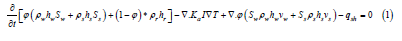
where ϕ is density, h is enthalpy, S is saturation of water, K_a is thermal conductivity, I is the identity matrix, T is temperature, v is interstitial velocity, and q_sh is the flow-rate intensity of an enthalpy source, and the subscripts w, s, and r, are water, steam, and rock, respectively. Assuming there is no steam in the system and the water stays in liquid form, all terms with subscripts will become 0, and the saturation of water in the liquid phase (Sw) will be equal to 1, giving:

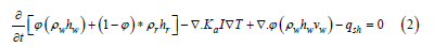
If fluid velocity in the pore spaces is assumed to be very slow, or zero (v_w=0) the equation again reduces further to:

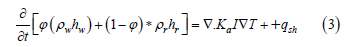
Equation 3 is applied by HYDROTHERM to the system by shutting off the terms given the value of zero. The program iterates through time-steps for either a transient or a steady state solution. From multiple algorithms available for solving each time step for pressure and temperature, the Newton Raphson method was selected, and the Crank-Nicholson time stepping calculation was used as it is unconditionally stable as compared to other implicit and explicit time stepping [45].

CSMHYD

Developed by Sloan in 1990, and updated in 1998 [31], CSMHYD is a code used to determine where gas hydrates are stable in the subsurface. The code determines the stability of the gas hydrates using a three phase equilibrium analysis of where the hydrates will form based on temperature, pressure, salinity, and gas composition [9]. Much of Sloan’s calculations are based on Barrer [41]. As discussed previously, there are three structure types for gas hydrates, based on the cage sizes associated with each type. Structure I and II clathrate hydrates have two different cage sizes, a small and a large. The two smaller structures are the same size for structure I and II, but the larger cage of Structure II is larger than that of the larger cage of Structure I. This changes the size of the gas molecule that is able to fit inside of the water cage. When the cages are filled with the appropriately sized molecules and enough of the cages are filled, the gas hydrates are stable [7]. The code determines the phase equilibrium based on gas hydrate composition, which determines the structure type, the temperature, and the effects of any inhibitor (such as salt) in order to produce a pressure that is in equilibrium with these factors to produce gas hydrate. The resulting pressure and temperature curve is the plot of the phase change between hydrate and free gas, as shown in Figure 3b, along with water for the 1-D model. Further description of the CSMHYD code is found in Sloan [31].

First, we constructed a velocity model based on the WesternGeco profiles. Then we built a salinity model. Using these models as input, we used the HYDROTHERM code to calculate a resulting thermal model. Finally, using the thermal and salinity models, we constructed a three-dimensional thermobaric model using CSMHYD.

Velocity Model

Through velocity analysis by WesternGeco, stacking velocity profiles were provided along with the seismic data (Figure 4).

These were converted to interval velocities using Dix Equation,

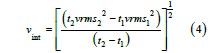
Figure 4:Interval Velocity Profiles at Station 156: a) interval velocity profile (in m/s) without smoothing the errors associated with converting from stacking velocity using Dix equation; and b) smoothed interval velocity profile using a box filter.

where v_int is the interval velocity, t is two-way travel time, and v_rms is the stacking velocity or true root mean square velocity. The interval velocity is the velocity over a depth interval and provides information about individual layers. Calculating the interval velocities can be complex because a minor change in the stacking velocity causes an anomalously high interval velocity, as shown in Figure (4a). Due to this, the calculated interval velocities were then smoothed (Figure 4b). The convolution operator was applied to the box filter, producing a triangle filter. The final velocity model covers an area greater than 57,700km². While it is larger than the region of interest, it allows for the depth conversion of the entire MC-118 lease block. In Figure 5 the stacking velocities for a 3D volume show an overall increase in velocity with depth, as was expected. The region where the southwest salt dome is located shows higher velocities than the surrounding sediments, and a velocity high located above the location of the salt dome. There is also a velocity high in the northeast portion of the MC-118 lease block, near the other salt dome located in the region.

Figure 5:3D Volume Stacking Velocities: 3D view of stacking velocities (in m/s) from the WesternGeco dataset. The x and y axes show locations in meters and the z-axis displays two-way travel time. The scale shows velocity where blue is slower, and read is higher velocity. The data shows an overall increase in velocity with depth.

The smoothed interval velocities (Figure 6), show a velocity high more than 1,000m/s greater than the sediments above and below located approximately 1,000m below seafloor in the northeast corner of MC-118 where a salt body is identified, and the area where the Woolsey Mound salt dome is located. The velocities at these areas gradually increase to the velocity difference of greater than 1,000m/s at the locations at the top of the salt domes. A large velocity spike much lower in the section is noted. Beginning at 6,000 to 7,000m below the seafloor, the velocity ranging from 1000–3000m/s greater than the surrounding sediment, and the remaining sediment below, reaching a velocity of 8,000m/s. This is likely the opal A to opal CT transition that marks the transformation of unconsolidated sediments to a more consolidated form, and highlighted with the horizontal slice in Figure 6.

Figure 6:3D Volume Smoothed Interval Velocities: 3D display of the smoothed interval velocities (in m/s) used in converting the location of the top of the salt.

Salinity model

Figure 7 shows the top of the salt dome as determined from seismic data. Using the velocity model, the salt tops were converted from two-way travel time to depth. A linearly increasing salinity gradient from the seafloor to the top of the salt was generated using two different salt concentration values, and assumed the majority of the salt in the diapir was NaCl.

Figure 7:Map of sea floor and top of Salt Diapir: Interpolated locations of the salt beneath the topography of MC118 based on the seismic, and converted to depth using the velocities. The top layer of topography shows depth beneath the sea surface.

i. Model 1 (53). The first salinity gradient ranged from sea floor salinity values to standard temperature pressure values of saturation, or 3.5-56% salt, where standard temperature and pressure are defined as 25 ⁰C and 1atm. Standard temperature and pressure conditions for the saturation point of salt were chosen for the first model because the saturation point of NaCl changes very little in response to both temperature and pressure. This was set as a minimum for what the concentration of salt had to be at the top of the salt dome, knowing that the true value would likely be much higher.
ii. Model 2 (90). The second gradient included values ranging from sea floor salinity to 90% salt, as the core of a salt dome is documented to be 90-99% salt [46]. These linearly varying salt concentrations produced a salinity gradient that changed with respect to how far the top of the salt dome was relative to the sea floor. The points over the salt dome span 2,900m by 2,650m, with 810 different salinity gradients within the area. It is widely understood that salinity does not linearly increase with depth, even in the presence of a salt diapir [47,48]. The salinity gradient is highly affected by the convection of lower density warm waters from deeper sources, and colder, denser waters found in the shallow subsurface. This mixing creates saline rich plumes of water as the salt from the outer region of the salt diapir is dissolved. Most likely, the salt concentrations will increase significantly closer to the salt dome and along the side of the salt diapir, but will remain relatively low in the shallower sediments [48].

Thermal model

In order to calculate the stability field of the gas hydrates, a model of the thermal environment was constructed based on the sedimentary properties derived through seismic interpretation, lithostratigraphic studies, and heat flow measurements in the shallow seafloor [23,25,26]. This is highly dependent on the salt diapirs located at the study site and the contrasting properties of the surrounding sediments. The salt alters the thermal environment due to its relatively high thermal conductivity. In order to model the thermal environment, the HYDROTHERM modeling code is used. HYDROTHERM can be used as a 1D, 2D, or 3D finite element code. This study interpolates a series of 2D seismic lines to create a 3D volume. To calculate the temperatures in the subsurface, the simplified heat flow equation uses the following:

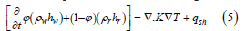
where ϕ is porosity, ρ density, h is enthalpy, t is time, k is permeability, T is temperature, q is heat source, and the subscripts w, r, and sh stand for fluid, rock/sediment, and enthalpy source, respectively. The HYDROTHERM modeling code also allows for pore waters to move through the system. But for the purposes of this research, the advection of fluids was not included. Therefore, the advection term of the heat flow equation is absent. The term remaining on the left hand side of the equation is the conduction term, which takes into account the density, porosity, and enthalpy of the water and the sedimentary medium. The fluid terms remained the same, and the rock/sediment terms changed based on whether they are salt or sediments. The source and sink terms are represented by qsh, where the source term is an average steady state basal heat flux in the Gulf of Mexico after Husson et al. [49].

In order to model the temperature, the Woolsey Mound was broken down into 30 different profiles running north to south that were spaced 100 meters apart from east to west (Figure 8). Figure 8a also shows where the salt has been interpreted in the southern region of MC118, with a color bar corresponding to the depth of the top of the salt. For each profile, a grid was discretized to span 2,700m, north to south, and 2,400m depth. The resulting grid was 48 by 48 cells, where the depth covered by each cell was 50m, and the horizontal distance was 100m (Figure 8b). The location of the salt and the sedimentary properties of the salt and surrounding sediments were then imported into their assigned cell. To simplify the calculations, the surrounding sediments were averaged to one type of sediment that combined the sedimentary properties of the interbedded sand and clays. This provided a model that would calculate the temperatures based on the salt in contrast with the overlying and surrounding sediments.

Figure 8:Slices of thermal model: a) Horizontal slice showing aerial extent of the area covered by the thermal model with a plot of where the salt is located and the depth at which it is located; and b) Vertical slice, or 2D profile, of the thermal model, set at initial conditions, prior to running the thermobaric model..

Figure 9 shows a vertical slice of MC-118, running from south to north, and cutting through the center of the salt dome. The model shows an increase in temperatures in the shallow sediments above the salt dome, as compared to the temperatures further away from the salt dome. Similarly, there was a decrease in temperatures below the salt dome, as compared to the temperatures deeper in the profile away from the salt. A clearly defined dome shape is present in the temperature profile where the salt is located. This pattern continued through all of the profiles that included the salt dome, with the curvature of the temperatures increasing upward in temperature at shallower depths most prominent at the crest of the salt dome. In the regions where the salt is absent, there are no temperature anomalies and the temperatures increase uniformly with depth, lacking the dome shape change in temperatures. This is indicated by a pseudo-3D temperature plot (Figure 10).

Figure 9:Profile of calculated temperatures at salt crest: Both plots show the final temperature output of the HYDROTHERM model over the shallowest part of the salt dome. The y-axis shows depth, down to 2,200m and the x-axis shows relative northing, where the northern most position is the right side of the plot. The dome shape appearance in the temperature profile is associated with the presence of salt, creating a thermal high. upper) 2D temperature model (in °C) with nodes of temperature after running the code to steady state conditions; and lower) temperatures imported into Matlab without the nodes.

Figure 10:3D volume temperature model: Pseudo 3D temperature plot with cooler temperatures represented by the blue color, and warmer colors increasing up the color bar to red, which is the warmest temperatures. The salt diapir is clearly delineated by the dome shape of increase temperatures in the profile along Relative Easting line 17 (the right most profile). The lack of salt creates a regular temperature distribution as seen in the profile furthest to the left, Relative Easting line 2.

Thermobaric model

Thermobaric modeling is the pressure and temperature stability modeling between phases in a given system. For gas hydrates, a thermobaric model maps the pressures and temperatures along which the phase change occurs between frozen gas hydrate and free gas. The 1998 version of Sloan’s CSMHYD code [31] was used to calculate the pressures where hydrates are stable based on salt concentrations and the gas composition at a given temperature. The salt concentrations and temperature values are discussed in sections 4.2 and 4.3. The thermobaric model uses the temperature and salinities to calculate a pressure necessary to create a stable environment for gas hydrate formation. Once the pressures are calculated, they can be converted to depth, based on a hydrostatic pore pressure gradient of 0.1atm/m [42,43]. Hydrates will form down to the depth where the thermobaric curve for hydrate stability intersects the geothermal gradient. The code itself can only calculate one depth point at a time for a given location, so a Matlab script was written to iteratively run the executable program for increasing depth points at varying locations. The area was defined using the same dimensions as the temperature and salinity models, resulting in a 3,000m by 2,700m area covered, with a total of 810 locations to be calculated. Two different models were calculated, each with different salinity assumptions to show how the salinity of the sediments affects the depth to the BGHSZ. Once the stability pressures were calculated and converted to depth, the thermobaric stability curve and geothermal gradient were graphed in order to find their intersection for the BGHSZ as described previously for (Figure 2 & 3). The depth of stability for each of the 810 locations were then plotted in an interpolated mesh grid.

For each of the two models (Figure 11 & 12), the estimated BGHSZ is located just below the topography, and above the salt diapir. The shape of the stability zones are a thinner dome shape with relationship to the shape of the salt dome. The depth of the BGHSZ calculated based on salt concentrations ranging from sea floor levels to STP is 140m, or 118m to 158m below the seafloor. The height of the BGHSZ calculated based on salt concentrations ranging from sea floor levels to 90 weight percent is 119m, or 67m to 186m below the seafloor. The shallowest stability values are at the crest of the salt dome and the deepest stability depths for the two models are at the edges of the salt dome as expected.

Figure 11:3D BGHSZ within subsurface at STP for salt: Map of the BGHSZ located beneath the mapped seafloor and above the salt diapir with a varying salt concentration ranging from sea water levels to standard temperature and pressure condition. The coloring of the layers is only shown to give perspective on the change in depth between the layers. The 3D image has been rotated to show a side view of the dome in relation to the topography and BGHSZ so the thickness of the stability zone below seafloor can be displayed

Figure 12:3D BGHSZ within subsurface for 90% salt: Map of the BGHSZ located beneath the mapped seafloor and above the salt diapir with a varying salt concentration from sea water levels to 90 weight percent salt. The coloring of the layers is only shown to give perspective on the change in depth between the layers. The 3D image has been rotated to show a side view of the dome in relation to the topography and BGHSZ so the thickness of the stability zone below seafloor can be displayed.

The Gulf of Mexico is a region known for its gas and oil resources as well as complex salt structures. This has made the mapping of the BGHSZ difficult through typical means that consists of locating a BSR in seismic sections. The salt disrupts the thermal environment by channeling heat through the sediments because of its high thermal conductivity. Salt also inhibits the formation of hydrates by lowering the free energy of water in the liquid phase. By accounting for salinity and temperature changes through thermobaric modeling, the BGHSZ can be estimated even without an obvious BSR present. In the presence of salt, we expect to see a thermal high at the shallowest point of the salt dome, and a thinning of the stability zone in the thermobaric model due to the higher temperatures and higher salinity gradient.

Modeling

Temperature has the greatest effect on gas hydrate stability as it prohibits the water molecule cages from forming. Figure 10 shows the temperature distribution at Woolsey Mound. The region where the salt dome is located shows an increase in temperature as compared to the surrounding sediments of the same depth. Similarly, the base of the salt diapir displays lower temperatures than that of the surrounding sediments. It is likely the high thermal conductivity of the salt preferentially funneled heat through the salt system, resulting in the temperature found. In the sediments where there is no salt dome, the temperatures increase at a near linear rate with depth because there is no change in the sediment properties to affect how the heat travels, and any nonlinear temperatures are a result of high heat flow associated with the fault. These affects lessen the further away from the salt diapir the sediments are. This also agrees with the high heat flow values from Macelloni et al. [25], where the mound system had much higher heat flow values than the sediments located away from the salt dome.

Figure 11 & 12 show a thin domed layer above the Woolsey Mound salt diapir located below. This is the base of the gas hydrate stability zone. As the salinity and geothermal gradient increase with the shallowing of the salt, the stability zone also shallows. This shallowing is a result of the salinity and temperature inhibiting the formation of the gas hydrates, because the water is unable to freeze and form the ice-like cages of water molecules. Figure 11 shows a thicker hydrate stability zone between the topography and the base of the stability zone as compared to Figure 12. The higher salinity gradient used in the calculation of Figure 12 causes this shallower stability zone. Based on the properties of salt, which lowers the free energy of liquid water, the shallower result is due to the higher weight percent salt used in Figure 12. Figure 11 shows a thicker stability zone because the lower salinity gradient has less of an effect on the temperature and hydrate formation. The model displays the properties of hydrates that were expected. An increase in the salinity and temperature blocks hydrate formation, and thins the region where they are stable. Both thermobaric models show this by having a dome shape as the salt diapir crests and also between the two models as the thinner stability zone is associated with a higher salinity gradient (Figures 11 & 12).

Future Directions and Caveats

The results of the thermobaric models (Figure 11 & 12) provide comparable results with the location of the BGHSZ indicated in a two-dimensional model by Macelloni et al. [25]. However, this is only a starting point for a more accurate three-dimensional model mapping the BGHSZ at MC-118. Two detailed models need to be created in order to place a better estimate on where the hydrates at Woolsey Mound are stable. A geologic model and a salinity model used to rerun the thermal and thermobaric models will aid in the accuracy. As stated, the sediments around the salt diapir were homogenized for the purpose of this study. A geologic model accounting for stratigraphic changes will allow for a more accurate calculation of the salinity and thermal models because the properties of the sediments themselves change how the salinity and temperature are distributed within the subsurface. The current model also disregards the role that faults play in the transport of heat, salinity, and gas. Including the location of the faults in a geologic model to allow for fluid motion in subsequent models would increase the overall accuracy in the estimation of the base of the gas hydrate stability zone.

A salinity model based on the properties determined in the geologic model and calculated using a program to model salt and fluid motion would capture a more realistic salinity gradient that changes with proximity to salt. Faults can act as conduits for the salt, unevenly distributing high salt concentrations to the sediments near the faults, while lack of convection can lead sediments away from the faults and above the salt dome low in salt concentration. Creating a nonlinear relationship between salt concentrations from the sea floor to the top of the salt dome will greatly enhance the prediction of the BGHSZ. Creating these two models, and then applying the geologic model to the simplified thermal model will allow for the advection and convection of salt and fluid through the entire system, especially through the faults. The updated salinity and thermal model will change the thermobaric model and is predicted to shallow the stability zone where faults and salt are moving and deepen the stability zone where there is no fluid motion to increase the temperature and salinity. Continuing the research in this direction will improve the accuracy of the thermobaric model and produce a better prediction of the BGHSZ.

Thermobaric modeling has been used in the past to determine where the BGHSZ is located in regions where BSRs are not present. Highly dependent on the thermal environment and the salinity gradient, a depth for the hydrate stability zone was determined to exist between 70 and 120m below the seafloor, at its shallowest point. These estimates corresponded with the nature of gas hydrates, as the hydrates were less likely to form in the areas of higher temperature and salinity. Constraining where these hydrates are stable is important for estimating the volume of gas resources and understanding the destabilization associated with the changes in their environment. This study was aimed at producing a 3D estimate of the BGHSZ based on temperature and salinity changes associated with salt diapirs. Our study extends model computation and mapping to a 3D thermobaric model for the base of the gas hydrate stability zone.

The authors would like to thank TGS-Nopec and WesternGeco for providing seismic data. We would like to also thank the USGS for use of the modeling code HYDROTHERM for heat flow calculation. The use of the hydrate stability code CSMHYD from Sloan (1998) is acknowledged. The research described here is substantially based on the work of Amanda Q. Williams for the Master of Science degree in Geology at the University of South Carolina, School of the Earth, Ocean, and Environment [50].

1. Collett TS, Lee MW, Zyrianove MV, Mrozewski SA, Guerin G, et al. (2012) Gulf of Mexico gas hydrate joint industry project leg ii logging-while-drilling data acquisition and analysis. Mar Petrol Geol 34(1): 41-61.
2. Kastner M, Myers M, Koh CA, Moridis G, Johnson JE, et al. (2022) Energy transition and climate mitigation require increased effort on methane hydrate research. Energy Fuels 36(6): 2923-2926.
3. Farahani MV, Hassanpouryouzband A, Yang J, Tohidi B (2021) Insights into the climate-driven evolution of gas hydrate-bearing permafrost sediments: Implications for prediction of environmental impacts and security of energy in cold regions. RSC Advances 11(24): 14334-14346.
4. Wu S, Bally AW, Cramex C (1990) Allochthonous salt, structure and stratigraphy of the North-Eastern Gulf of Mexico. Part II: Structure. Mar Petrol Geol 7(4): 318-333.
5. S. Department of State (2007) Projected greenhouse gas emissions. In: Fourth climate action report to the UN framework convention on climate change.
6. Aresta M, Dibenedetto A, Quaranta E (2016) Thermodynamics and applications of CO₂ In: Reaction mechanisms in carbon dioxide conversion. Springer Publishers, UK, pp. 373-402.
7. Buffett BA (2000) Clathrate hydrates. Annu Rev Earth Planet Sci 28: 477-507.
8. Kvenvolden KA, Ginsberg GD, Soloviev VA (1993) Worldwide distribution of subaquatic gas hydrates. Geo-Marine Lett 13(1): 32-40.
9. Sloan ED (1990) Clathrate hydrates of natural gas. Marcel Decker Inc. Publishers, USA.
10. Ruppel CD, Kessler JD (2016) The interaction of climate change and methane hydrates. Reviews of Geophysics 55(1): 126-168.
11. Ruppel C, Dickens GR, Castellini DG, Gilhooly W, Lizarralde D (2005) Heat and salt inhibition of gas hydrate formation in the northern Gulf of Mexico. Geophysical Research Letters 32(4): LO46605.
12. Makogon YF, Makogon F (1997) Hydrates of Hydrocarbons. 1^st (Edn.), PennWell Books, USA, pp. 1-482.
13. Alam S, Knapp C, Knapp J (2024) Three-dimensional amplitude versus offset analysis for gas hydrate identification at Woolsey Mound: Gulf of Mexico. GeoHazards 5(1): 271-285.
14. Hyndman RD, Spence GD (1992) A seismic study of methane hydrate marine bottom simulating reflectors. J. Geophys Res 97(B5): 6683-6698.
15. Singh SC, Minshull TA, Spence GD (1993) Velocity structure of a gas hydrate reflector. Science 260 (5105): 204-207.
16. Helgerud MB, Dvorkin J, Nur A, Sakai A, Collett T (1999) Effective wave velocity in marine sediments with gas hydrates: Effective medium modeling. Geophys Res Lett 26(13): 2021-2024.
17. Shedd W, Boswell R, Frye M, Godfriaux P, Kramer K (2012) Occurrence and nature of “bottom simulating reflectors” in the northern Gulf of Mexico. Mar Petrol Geol 34(1): 31-40.
18. Sloan ED, Koh C (2008) Clathrate hydrates of natural gases. 3^rd (Edn.), CRC Press, USA, pp. 1-756.
19. Liu X, Fleming PB (2007) Dynamic multiphase flow model of hydrate formation in marine sediments. J Geophys Res 112(B3): 1-23.
20. Shipley TH, Houston MH, Buffler RT, Shaub FJ, McMillen KJ, et al. (1979) Seismic evidence for widespread possible gas hydrate horizons on continental slopes and rises. AAPG Bulletin 63: 2204-2213.
21. Sassen R, Roberts HH, Jung W, Lutken CB, DeFreitas DA, et al. (2006) The Mississippi Canyon 118 gas hydrate site: A complex natural system. Offshore Technology Conference, USA.
22. Lapham LL, Chanton JP, Martens CS, Sleeper K, Woolsey JR (2008) Microbial activity in surficial sediments overlying acoustic wipeout zones at a Gulf of Mexico cold seep. Geochem Geophys Geosyst 9(6): Q06001.
23. Macelloni L, Simonetti A, Knapp JH, Knapp CC, Lutken CB, et al. (2012) Multiple resolution seismic imaging of a shallow hydrocarbon plumbing system, Woolsey Mound, Northern Gulf of Mexico. Mar Petrol Geol 38(1): 128-142.
24. Simonetti A, Knapp JH, Knapp CC, Macelloni L, Lutken CB (2011) Defining the hydrocarbon leakage zone and the possible accumulation model for marine gas hydrates in a salt tectonic driven cold seep: Examples from Woolsey Mound, MC118, northern Gulf of Mexico. Proceedings of the 7^th International Conference on Gas Hydrates (ICGH 2011), UK.
25. Macelloni L, Lutken CB, Garg S, Simonetti A, D’Emidio M, et al. (2015) Heat-flow regimes and the hydrate stability zone of a transient, thermogenic, fault-controlled hydrate system (Woolsey Mound northern Gulf of Mexico). Mar Petrol Geol 59: 491-504.
26. Simonetti A, Knapp JH, Sleeper K, Lutken CB, Macelloni L, et al. (2013) Spatial distribution of gas hydrates from high-resolution seismic and core data, Woolsey Mound, Gulf of Mexico. Mar Petrol Geol 44: 21-33.
27. Wood WT, Hart PE, Hutchinson DR, Dutta N, Snyder F, et al. (2008) Gas and gas hydrate distribution around seafloor seeps in Mississippi Canyon, Northern Gulf of Mexico, using multi-resolution seismic imagery. Mar Petrol Geol 25(9): 952-959.
28. Salvador A (1987) Late Triassic-Jurassic paleogeography and the origin of the Gulf of Mexico basin. AAPG Bulletin 71(4): 419-451.
29. Ingram WC, Meyers SR, Brunner CA, Martens CS (2010) Late pleistocene–holocene sedimentation surrounding an active seafloor gas-hydrate and cold-seep field on the Northern Gulf of Mexico slope. Marine Geology 278(1-4): 43-53.
30. Wilson SJ, Hunter RB, Collett TS, Hancock S, Boswell R, et al. (2011) Alaska North slope regional gas hydrate production modeling forecasts. Mar Petrol Geol 28(2): 460-477.
31. Sloan ED (1998) Clathrate hydrates of natural gas. 2^nd (Edn.), Marcel Decker Inc. Publishers, USA.
32. Trehu AM, Ruppel C, Holland M, Dickens GR, Torres ME, et al. (2006) Gas hydrates in marine sediments: Lessons from scientific ocean drilling. Oceanography 19(4): 124-142.
33. Diaconescu CC, Kieckhefer RM, Knapp JH (2001) Geophysical evidence for and thermobaric modeling of gas hydrates in the deep water of the South Caspian Sea, Azerbaijan. Mar Petrol Geol 18(2): 209-221.
34. Diaconescu CC, Knapp JH (2000) Buried gas hydrates in the deepwater of the South Caspian Sea, Azerbaijan: Implications for geo-hazards. Energy Exploration and Exploitation 18(4): 385-400.
35. Xu W (2004) Modeling dynamic marine gas hydrate systems. American Mineralogist 89: 1271-1279.
36. Mienert J, Vanneste M, Bünz S, Andreassen K, Haflidason H, et al. (2005) Ocean warming and gas hydrate stability on the mid-Norwegian margin at the Storegga Slide. Mar Petrol Geol 22(1-2): 233-244.
37. Bangs NL, Musgrave RJ, Tréhu AM (2005) Upward shifts in the south hydrate ridge gas hydrate stability zone following post-glacial warming offshore Oregon. J Geophys Res 110(B3): 13.
38. Ruppel C (2000) Thermal state of the gas hydrate reservoir. In: Max MD (Ed.), Natural Gas hydrate in oceanic and permafrost environments. Kluwer Academic Publishers, USA, pp. 29-42.
39. MacDonald IR, Guinasso NI, Sassen R, Brooks JM, Lee L, et al. (1994) Gas hydrate that breaches the seafloor on the continental slope of the Gulf of Mexico. Geology 22(8): 699-702.
40. MacDonald IR, Bender LC, Vardaro M, Bernard B, Brooks JM (2005) Thermal and visual time-series at a seafloor gas hydrate deposit on the Gulf of Mexico slope. Earth Planet Sci Lett 233(1-2): 45-59.
41. Barrer RM, Stuart WI (1957) Non-stoicheiometric clathrate compounds of water. Proceedings of the Royal Society of London. Series A, Mathematical and Physical Sciences 243(1233): 172-189.
42. Kvenvolden KA, Barnard LA, Brooks JM, Wiesenburg DA (1981) Geochemistry of natural-gas hydrates in oceanic sediment. In: Bjoroy M, (Ed.), Advances in Organic Geochemistry, Online Wiley Publishers, UK, pp. 422-430.
43. Kvenvolden KA (1993a) A primer on gas hydrates. In: Howell DG (Ed.), The future of energy gases. U. S. Geological Survey Professional Paper, 1570: 279-291.
44. Kvenvolden KA (1993b) Gas hydrates as a potential energy resource –A review of their methane content. In: Howell DG (Ed.), The future of energy gases. U. S. Geological Survey Professional Paper, 1570: 555-561.
45. Kipp KL, Hsieh PA, Charlton SR (2008) Guide to the revised ground-water flow and heat transport simulator: HYDROTHERM — Version 3. U.S. Geological Survey Techniques and Methods 6−A25, pp. 1-160.
46. Hart P, Johnson RL, Nicholson TJ, Quinn E, Wright RJ (1981) US Nuclear Regulatory Commission. Survey of Salt Dome investigations, pp. 1-58.
47. Smith AJ, Flemings PB, Fulton PM (2014) Hydrocarbon flux from natural deepwater Gulf of Mexico vents. Earth Planet Sci Lett 395: 241-253.
48. Jamshidzadeh Z, Tsai FTC, Ghasemzadeh H, Mirbagheri SA, Barzi MT, et al. (2015) Dispersive thermohaline convection near salt domes: A case at Napoleonville Dome, Southeast Louisiana, USA. Hydrogeol J 23: 983-998.
49. Husson L, Pichon XL, Henry P, Flotte N, Rangin C (2008) Thermal regime of the NW shelf of the Gulf of Mexico Part B: Heat flow. Bull Soc Géol Fr 179(2): 139-145.
50. Williams AQ (2016) Three dimensional thermobaric modeling of a gas hydrate system. Master of Science Thesis, University of South Carolina, USA, pp. 1-44.