Comparison Linear Programming and Improving Shuffled Complex Algorithm for Optimizing Multi Reservoir Systems

Taking into account the constraints of water resources and the fact that the total amount of water on earth is constant, exploitation of the reservoir is one of the key issues among the various issues of water resources. As a result, the application of optimization techniques is required to determine the utilization plan of the reservoirs. Oliveira & Loucks [1] used the genetic algorithm to optimize the parameters of the exploitation policy in a multi-reservoir system [1]. Asfaw and Hashim used a genetic algorithm to optimize hydroelectricity [2]. Tayebian et al. [3] reviewed the performance of the genetic algorithm in order to optimize the hydrogeological reservoir exploitation policy to maximize the hydroelectric power generation. Their results showed that using this algorithm increases the hydroelectric power generation and increases the system stability [3]. Moradi & Dariane [4] improved the performance of the PSO algorithm by using the genetic algorithm mutation operator, and then used the improved algorithm to solve a single-reservoir and single-objective problem [4]. Mousavi et al. [5] used the PSO algorithm to solve the problem of optimum use of hydroelectric power [5]. Ghimire and Reddy used the PSO algorithm to extract optimum policies for the exploitation of a single reservoir hydrophobic system [6]. Afshar et al. [7] used the Honey-Bee Mating Optimization (HBMO) to optimize the exploitation of the Dez Dam reservoir. The results showed that the efficiency and performance of this algorithm are very suitable for convergence to absolute optimum response [7]. In an exploratory study of the optimum utilization problem of the hydroelectric multi-reservoir system, Haddad et al. [8] showed the effectiveness of HBMO to find the best solution in comparison to the classic NLP method performed by LINGO 8.0 [8].

DE algorithm is an intelligent and population-based optimization algorithm [9,10]. In the field of exploitation of reservoir, Yin & Liu [11] addressed the problem of optimizing the amount of hydroelectric power generation from a single-reservoir system using DE algorithm [11]. The Shuffled Complex Algorithm (SCE) is a global search algorithm [12]. Many researchers have proved the great abilities and power of the SCE algorithm, especially in the calibration of rainfall-runoff models [13,14]. Contrary to the widespread use of this highly potent algorithm in various issues, SCE algorithm has been rarely used to solve the problems of optimizing the reservoirs; and has not been well-proven in solving complex water resources issues. Nazhad et al. [15] evaluated the performance of the SCE-DE algorithm for two-reservoir system. They found that optimization by SCE-DE is much better than SCE algorithm [15].

According to a review conducted on published papers regarding the subject of this study, it is concluded that all of them have investigated the SCE algorithm and DE algorithm for single or two- reservoir systems. In the current research, for the first time, the SCE algorithm is improved through the integration with the DE algorithm to optimize complex water resources problems based on continuous 4-reservoir systems. In addition, the results are compared with those of the LP method. To this end, the SCE algorithm is integrated with the DE algorithm through the coding process in MATLAB. Also, to evaluate the performance of three benchmark mathematical function problems solved by this improved algorithm (SCE-DE), they are compared with the original SCE algorithm. Then, to investigate the performance of these algorithms in solving complex water resource optimization problems, an example of continuous 4-reservoir systems is solved, and the answers are compared with those of the LP method.

Shuffled Complex evolutionary Algorithm (SCE)

The Shuffled Complex Evolutionary Algorithm (SCE) is a global search algorithm [16] which is based on the best features of several existing algorithms, including the genetic algorithm and the introduction of the concept of composition of communities. The general description of the SCE algorithm and its various steps are presented below:

a) Creating a sample: Create a random sample (S point) in the available space and obtaining the function value in each point.

b) Sorting: Sort S points in ascending order in an array such as D: D = {(xi, fi), i = 1,2, ..., s}

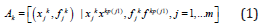
c) Classifying sample points S into P community so that each community has m points. In fact, D is converted to the communities A₁, A₂, ..., Ap, each of which has m points, namely:

d) Developing each community, A and X = 1,2, ..., P based on Competitive Complex Evolution (CCE) algorithm.

e) Reshuffling the points of different communities so that there is only one instance of the points, that is, the communities A₁, A₂, ..., A_p again are substituted in D array and then are sorted based on the ascending values.

f) Reviewing convergence: Stop the program if any of the convergence criteria is met.

g) Otherwise, go back to step three and run calculations.

Differential Evolution (DE) algorithm

The differential evolution algorithm is a population-based optimization algorithm. This algorithm was first introduced by Storm & Prince [17]. The mutation operator as follows:

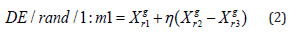
In previous equations, r₁≠r₂≠r₃ is the index of randomly selected vector, η∈[0.2,0.8] is a random number of a uniform distribution, V_i,g+1 is the best vector with the best objective function. Then mutation operator is A_pplied on vector V_i,g+1 and the new vector V_i,g+1 is created. There are the corresponding equations below:

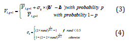
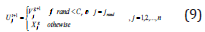
In the above equations, rand is a random number between [0,1]. The parameters of distribution β and the rate of mutation p are both controlling parameters. Lb and Ub are the minimum and maximum decision variables, respectively.

To apply the intersection operator, consider the vector V_i,g+1 created by mutation operator, then apply the following equation to obtain the intersection vector U_i,g+1.

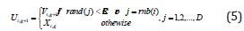
In (8), rand (j) is the jth value of a random number between [0,1]. CR is intersection factor between [0,1]. Rnb (i) is a random variable of 1, 2, ... D. (D is the dimension of the problem decision variables) to ensure that at least one parameter is selected from vector V_i,g+1

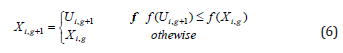
This operator states whether the vector i,g 1 U + must be a member of the next-generation population (g + 1). In this case, the obtained values of the objective function for two vectors, U_i,g+1, and X_i,g are compared with each other. If one assumes that the object of problem is minimizing, the vector X_i,g+1, which represents a vector in the next generation, is determined from the following equation.

Shuffled Complex Evolution and Differential Evolution (SCE-DE) algorithm

In this research, DE algorithm is used to improve the SCE algorithm, in a way that the DE algorithm helps to upgrade the performance, contraction operators, and reflection of the SCE algorithm. Here’s how this combination is. The exponential diagram of this method is also shown in Figure 1.

Figure 1:

1. Determining the initial values of the combined algorithm parameters (q, α, β, Cr and F).

2. Determining the probable values of each of the members in A using the following equation:

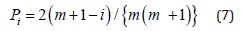
3. Where, m denotes the number of members in each community. Selecting q members from members A using the above equation, and then placing these members in the array B ={ u_i, v_i, i = 1,.......,q } where vi is equal to the value of the objective function at the point u_i.

4. Producing Children

A) Generating a mutated member from members of B using the following equation:

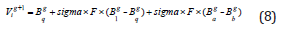
Where v^g+1_i is a mutated member? σ is fixed number usually chosen in the interval [1-2]. F is known as a mutation vector factor and F> 0. B^g_i is the ith member of the array B.B^g_a and B^g_q are best and worst members of array B, respectively.

B) Generating a member which is obtained through the intersection operator:

After the mutation operator, a new member is created by combining the mutated member and the ith member of the population 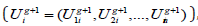which is described below:

5. If U_i^g+1 is within the allowed range of variables, calculate the value of its function (fz) and go to step 6, otherwise go to step 7.

6. If fz < fq, then replace the value of B^g_q with the value of U_i^g+1 and proceed to step 10; otherwise, go to step 7.

7. Calculate a new member by using an equation in which r is reflection of U_i^t+1 .

8. If r is within the allowed range of variables, calculates the value of its function (fr) and go to step 9; otherwise, generate a new member randomly, called and its function value is called fy.

9. If fr < fq then replace r with y, and proceed to step 10, otherwise, generate a new member randomly, called y, and its function value is called fy.

10. Repeat steps 2 to9 as α times.

11. Then, replace the new population generated in array B with the previous population and arrange them based on their objective function’s values.

12. Repeat steps 2 to 11 as β times.

Verification of the SCE-DE

In order to evaluate the ability of SCE-DE to find the optimal point, three benchmark functions with the specifications of Table 1 were investigated. The absolute optimal value of these functions is zero which is considered in this research as 30 dimensional functions. The number of objective function evaluations was assumed to be 10,000. 10 runs are performed for each function, and Figures 2-4 illustrate how the SCE and SCE-DE algorithms converge. Further Table 2 shows the target function values for these functions. As can be seen, the SCE-DE performs better than the SCE. In all functions, even the worst SCE-DE performance was better than the best SCE performance. The standard deviation of the SCE-DE solutions is less than the SCE, which is a strong point for the SCE-DE algorithm. The results show the high accuracy and proper performance of the SCE-DE algorithm in finding the optimal solution (Table 3 & 4).

Figure 2:

Figure 3:

Figure 4:

Table 1:

Table 2:

Table 3:

Table 4:

Continuous four-reservoir system

Chow & Cortes [18] first designed and solved the problem of using the continuous four-reservoir system [18]. In this hypothetical issue, the studied system consists of four reservoirs that are parallel and series according to Figure 5, in which the release of each reservoir is used to generate hydroelectric power. In addition, the release of reservoir number 4 is used to supply irrigation requirement. In this regard, the profit from supplying these two purposes is a linear function of the release rate, whose value is presented quantitatively as input of the problem. The operating period is 12 months.

In this regard, in equation (11), the matrix of the coefficients of relationship between the four reservoirs is presented in Figure 5.

Figure 5:

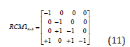
Where RCM_(4×4) is the matrix of the coefficients of relationship between the four reservoirs in the problem of exploiting four reservoir systems. As the aim of solving objective function in this problem is to maximize the function value, objective function is based on optimum release, and it is shown in equation (12).

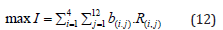
Where b_(i,j) is the values of the profit coefficients that are presented in Table 5. i is the number of reservoir and j is the number of periods. As with all the issues of exploitation of the reservoirs, the most important constraint on problem is the continuity relation, which is defined more simply according to equation (13) in hypothetical exploitation of the reservoir.

Table 5:

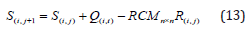
Q_(i,j) is the flow of input into the reservoir, R_(i,j) is the amount of release, and S_(i,j) is the volume of the reservoir? For all reservoirs, the constraints relate to the release and volume of the reservoir is according to equations (14) and (15).

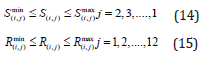
In the above equations, min S^min_(i,j) and S^max_(i,j) , are minimum and maximum storage of the reservoir, respectively. min R^min_(i,j) and R^max_(i,j) are the minimum and maximum release volume of the reservoir, respectively. The conditions for using the continuous four reservoir system are presented in accordance with Table 3. The maximum storage volume for each one of the four reservoirs of the above problem is different per month, and the information is presented in Table 4. The information about Inflow’s data in every period for each reservoir is provided in Table 6.

Table 6:

This challenging issue of water resources has been analyzed many a time. Chow & Cortes [18] have first designed and solved the problem of exploitation of continuous four-reservoir system. The optimum amount of objective function is 308.26 using LP method [18,19]. Later, Murray & Yakowitz [17] used DDP method for solving the mentioned problem and reported the optimum amount of objective function as 308.23 after eight repetitions which have 0.01% difference with that of Chow & Cortes [18]. They also reported 307.97 for 20 repetitions using DDDP method [19]. On the other hand, Haddad et al. [20] conducted a study and utilized LP method to solve the problem of continuous fourreservoir system and they reported 308.29 for the final response of objective function being different from that of Chow & Cortes [18]. In addition, Haddad et al. [8] used HBMO for solving the mentioned problem and reported 308.24 for optimum response and it is 0.02% lower than response in LP method (308.29) [20]. Jalali [19] solved this problem through ACO algorithm by considering 3000 repetitions and 200 ants so that the best response was 307.24 for this continuous state [21]. Through HAS algorithm after 1,000,000 repetitions, the optimum response was 307.218 [22]. In various projects, the optimum responses were 306.920, 308.20 and 308.28 using WCA, BA, and BBO algorithms respectively [23-25]. Moghari et al. analyzed GA, CIA and COA algorithms for this problem which resulted in 302.42, 306.76 and 307.92 optimum responses [26]. The solution of this problem has been reached 308.15 response using WOA algorithm [26].

In the present research, the result of objective function is 308.29 using LINGO 8.0 which is the outcome of using LP method being the absolute optima of this problem. To solve the problem by SCE and SCE-DE, the preliminary sensitivity of parameters has been analyzed for each of the methods and the results of best values selected have been presented in Table 7. Table 8 reports the results of objective function for 10 SCE and SCE-DE independent executions. As it can be seen, the best optimum response resulted of SCE has 1.84% difference from that of the LP method; but the best optimum response of SCE-DE method has 0.009% difference from that of the LP method. As a result, SCE-DE outperforms the SCE in reaching the most optimum value of fitness function. The convergence diagrams SCE-DE in Figure 2-4 has more convexity than major SCE diagrams in achieving the final optimum response. In fact, SCE-DE has proceeded with lower slope than two other algorithms in reaching the optimum response. According to Figure 6, the difference of final results in SCE-DE is low and the algorithm is reliable because SCE-DE has been reached the near-optimum response through more limited executions (based on number of assessment times).

Figure 6:

Table 7:

Table 8:

Release volumes for the best execution of continuous fourreservoir problem resulted from SCE and SCE-DE methods versus the release volumes resulted from LP method has been given in Figure 7. As it can be observed, SCE release volumes have considerable difference with LP. On the other hand, SCE-DE release volumes are compatible with the LP release diagram in many periods and reservoir releases. Release volumes of reservoir in the continuous four-reservoir problem have been shown in Figure 8 which belongs to the best execution of SCE and SCE-DE. As it can be seen, the calculated storages in both methods have been in the allowed range between minimum storage and maximum storage. Hence, the compatibility of SCE-DE storage volumes with LP storage volumes is more than the compatibility of SCE storage volumes with LP storage volumes. This fact points to the higher effectiveness of SCE-DE in solving the continuous four-reservoir problem. In this study, to evaluate different algorithms, we used the MAE, RMSE and correlation coefficients (R) between computational values with the LP response. Amount of MAE in SCE and SCE-DE were obtained 7.66 and 0.29 respectively. Furthermore, RMSE for the above algorithms were equal 7.78 and 0.53 respectively. The correlation coefficients in all algorithms were more than 99%.

Figure 7:

Figure 8:

In this research, SCE algorithm has been first merged with the DE algorithm to promote the SCE algorithm for being applied in the optimization and the algorithm generated was named as SCE-DE. Then, Ackley function was solved by two original SCE and promoted SCE-DE algorithms. The results show the superiority of SCE-DE algorithm in optimization. Then, for analyzing the performance of created algorithm and its evaluation in the complex problems of water resources, the hypothetical and challenging continuous four-reservoir problem which has been analyzed through different optimization algorithms was solved and the results of major SCE algorithm, and proposed SCE-DE algorithm with the LP results. In the continuous four-reservoir problem, the results indicate that SCE-DE performance is more optimal than that of SCE in reaching the LP response. The comparison shows that the proposed algorithm in this research (SCE-DE) possesses better performance in contrast to SCE algorithm. Also, Meanwhile, in comparing the solution of this complex multi-reservoir with the prior researches, very close responses to absolute optima has been achieved using HBMO, HAS, WCA, GA, ICA, COA, and WOA algorithms which by and large shows the very well performance of this algorithm in solving the problems of water resources optimization. Further the results of this research and the improved algorithm can be used in the energy production industry and in the optimization of the energy management of hydroelectric power plants. This improvement in the SCE algorithm enables the addition of hydroelectric power optimization in future work by further improving the algorithm in agricultural optimization work.

1. Oliveira R, Loucks DP (1997) Operating rules for multireservoir systems. Water Resources Research 33(4): 839-852.
2. Asfaw TD, Hashim AM (2011) Reservoir operation analysis aimed to optimize the capacity factor of hydroelectric power generation. International Conference on Environment and Industrial Innovation, pp. 28-32.
3. Tayebian A, Mohammed Ali TA, Ghazali AH, Malek MA (2016) Optimization of exclusive release policies for hydropower reservoir operation by using genetic Algorithm. J Water Resource Management 30: 1203-1216.
4. Moradi A, Dariane A (2009) Particle swarm optimization: application to reservoir operation problems. Advance Computing Conference, pp. 1048-1051.
5. Mousavi SJ, Shourian M (2010) Capacity optimization of hydropower storage project using particle swarm optimization algorithm. Journal of Hydro Informatics 12(3): 275-291.
6. Ghimire BN, Reddy MJ (2013) Optimal reservoir operation for hydropower production using particle swarm optimization and sustainability analysis of hydropower. ISH Journal of Hydraulic Engineering 19(3): 196-210.
7. Afshar A, Bozorg H, Mariño M, Adams BJ (2007) Honey-bee mating optimization (HBMO) algorithm for optimal reservoir operation. J Franklin Inst 344: 452-462.
8. Haddad OB, Afshar A, Mariño MA (2008) Design-operation of multi-hydropower reservoirs: HBMO approach. Water Resources Management 22(12): 1709-1722.
9. Storn R, Price K (1995) Differential evolution a simple and efficient adaptive scheme for global optimization over continuous spaces. International Computer Science Institute, Berkley, Greenwich, Connecticut, USA.
10. Storn R, Price K (1997) Differential evolution a simple and efficient heuristic for global optimization over continuous spaces. Journal of Global Optimization 11(4): 341-359.
11. Yin L, Liu X (2009) Optimal operation of hydropower station by using an improved DE algorithm. International Computer Science and Computational Technology (ISCSCT’09): 071-074.
12. Duan QY, Gupta VK, Sorooshian S (1993) Shuffled complex evolution approach for effective and efficient global minimization. Journal of Optimization Theory and Applications 76(3): 501-521.
13. Xiamong S, Chang Z, Jun X. (2011) Integration of a statistical emulator approach with the SCE_UA method for parameter optimization of a hydrological model. Chinese Science Bulletin 57(26): 3397-3403.
14. Dongmei X, Wang W, Chau K, Cheng CH, Chen SH (2013) Comparison of three global optimization algorithms for calibration of the xinanjiang model parameters. Hydro Informatics 15: 174-193.
15. Gen M, Cheng (1997) Genetic algorithm and engineering design.
16. Chow VT, Cortes R (1974) Applications of DDDP in water resources planning. Ideals.
17. Murray DM, Yakowitz SJ (1979) Constrained differential dynamic programming and its application to multireservoir control. Water Resources Research 15(5): 1017-1027.
18. Bozorg H, Afshar A, Mariño MA (2010) Multireservoir optimisation in discrete and continuous domains. Proc ICE Water Manag 164(2): 57-72.
19. Jalali MR (2005) Optimum design and operation of hydro systems by ant colony optimization algorithms; A new metaheuristic approach. Civil Engineering, Iran University of Science and Technology, Iran.
20. Kougias I, Theodossiou N (2011) Optimization of multi-reservoir management using Harmony Search Algorithm (HSA). Intern Conf on Environmental Management.
21. Bozorg H, Moravej, Loaiciga (2015) Application of the water cycle algorithm to the optimal operation of reservoir systems. J Irrig Drain Eng 141(5):
22. Bozorg H, Karimirad, Seifollahi A, Loáiciga HA (2014) Development and application of the bat algorithm for optimizing the operation of reservoir systems. J Water Resour Plan Manag 141(8):
23. Bozorg H, Hosseini M, Loáiciga SM (2015) Biogeography-based optimization algorithm for optimal operation of reservoir systems. J Water Resour Plan Manag 142(1):
24. Hosseini M, Morovati SM, Moghadas R, Araghinejad M (2015) Optimum operation of reservoir using two evolutionary algorithms: Imperialist Competitive Algorithm (ICA) and Cuckoo Optimization Algorithm (COA). Water Resour Manag 29(10): 3749-3769.
25. Asgari HR, Bozorg H, Pazoki M, Loáiciga HA (2015) Weed optimization algorithm for optimal reservoir operation. Journal of Irrigation and Drainage Engineering 27: 142.
26. Bakhtiari N, Najarchi O, Najafizadeh M, Mirhosseini H (2017) Developing a shuffled compelex evaluion algorithm using a differentiol evolution algorithm for optimizing hydropower reservoir systems. Water Supply 18(3): 1081-1092.