Modelling Zero-inflated Bivariate Count Responses using Marginal-Conditional Approach with application to Traffic Accidents and Fatalities Data

The problem of the presence of excessive zero values in the response variables is one of the major concerns in modeling count data. This problem arises in various fields such as biosocial science Long et al. [1], ecological studies Wang et al. [2], fishery studies Arab et al. [3] and Smith et al. [4] health studies Neelon et al. & Morgan et al. and Kassahun et al. [5-7] traffic accidents studies Papageorgiou, Meintanis [8,9] and the references therein. This characteristic of the presence of excessive zeros in the count data poses considerable challenges while modelling such data. Another issue of concern is the overdispersion stemming from the count data if the variance of the count responses is greater than mean, which might be attributed by excess zeros in the data. Since the work of Lambert [10], several models have been proposed to take account of the zero inflation in the count data in various fields, however, the problem with bivariate zero inflated models have not been discussed extensively in the literature.

Our work is motivated by two traffic accidents data sets. In the first data set, the daily number of accidents and the corresponding number of fatalities were investigated by Virginia state police between January 1, 1969 and October 31, 1970 Leiter & Hamdan [11]. In the second data set, the number of monthly accidents and corresponding fatalities were recorded between January 1997 and December 2004 in Groningen, The Netherlands Meintanis [9]. In both of these data sets, the first response variable represents number of accidents occurred during a particular time period. As there may not have any occurrence of accidents in a given time period, the first response variable i.e. number of traffic accidents may suffer the presence of excessive zeros. The second variable represents the count responses of the number of fatalities at a given time period related to the traffic accidents at that specific time period.

If the response of the first variable is zero i.e. no traffic accident occurs, the response of the second variable i.e. number of fatalities will also be zero. However, if the response of the first variable is non-zero, the response of the second variable still may be zero as the occurrence of accidents do not necessarily mean the occurrence of fatalities. Thus, the outcomes of the second response variable are conditionally related to the outcome of the first response variable. To model this type of data, one may require a modelling technique using an extended generalized linear model approach on the basis of marginal and conditional distributions to express the joint distribution of the Poisson outcomes for both the marginal and conditional variables. The use of the generalized linear model in this context makes the inferential procedures easier.

The bivariate Poisson regression models have been developed to address an increasingly important area of research with wide range of applications [12-15] in various fields where paired count data are correlated. Leiter & Hamdan [11] suggested bivariate probability models such as Poisson-binomial and Poisson-Poisson, with application to the traffic accidents and fatalities data. Following their approach, Cacoullos & Papageorgiou [16] proposed an alternative Poisson-binomial approach to model the relationship between the number of accidents and number of fatalities. Later Cacoullos & Papageor-giou [17] proposed a negative binomial-Poisson approach to analyze traffic accidents. The maximum likelihood approach-based parameter estimation techniques for negative binomial-Poisson models with their properties were proposed by Papageorgiou & Loukas [8]. Meintanis [9] proposed goodness-of-fit test procedures applicable to traffic accident data. Several other studies also reviewed and examined bivariate Poisson distribution in the literature Holgate, Consul, Consul , Consul & Shoukri [18-21].

Based on the Poisson-Poisson distribution proposed by Leiter [11], a bivariate generalized model is developed by Islam & Chowdhury [15] where the link functions are obtained for the bivariate Poisson model and inferential procedures are shown. As the zero-inflated responses restrict the use of the above described modelling approaches available in the literature, a further improvement of the model is essential to take account of the excessive zeros in the bivariate count data. Univariate zero-inflated Poisson (ZIP) model was extended to bivariate ZIP by Li et al. [22] to model the mixture of bivariate Poisson distribution and a point mass at (0,0).

Their approach was further extended with the application to workplace injury data by Wang et al. A bivariate Poisson-Poisson regression model was proposed by Cheung & Lam [5] using the bivariate Poisson distribution by Holgate [18] applicable to bimodal distributions of counts with one mode at zero. Their bivariate Poisson-Poisson ZIP model was also extended under this constraint that Response 1 ≥ Response 2. But the setup of our data set is different than the methodologies available in the literature. This is because, in the traffic accident data if Response 1 (number of accidents) is zero, then Response 2 (number of fatalities) has to be zero as well.

Thus, one needs to incorporate this constraint while modelling such data set. Consequently,  in this paper, we introduce a bivariate Poisson generalized linear model suitable for zero heavy count data with applications to traffic accident data. Our proposed approach is more general as it is based on the marginal and conditional distributions of two count variables where the marginal distribution of the first variable and the conditional distribution of the second variable for given value of the first variable follow Poisson distributions. The proposed model is expressed in exponential form and the link functions are obtained for generalized linear model of the bivariate Poisson outcomes and zero-inflation is taken into account for both the count outcomes. Although we illustrate the proposed approaches in two traffic accidents data sets, our approach is rather general and can be employed in other areas as well. For example, in health studies, the number of medical conditions diagnosed by the doctors for a group of patients and the number of health care facilities used by  that group   of patients may be an example of using a such modelling approach.

The plan of this paper is as follows. After introducing the bivariate zero-inflated Poisson model in Section 2, we provide the estimation techniques of the model parameters in Section 3. Application of the proposed model to the traffic accidents and fatalities data is presented in Section 4 and some concluding remarks are presented in the Section 5.

In this section we introduce a marginal-conditional approach based bivariate zero-inflated Poisson-Poisson model for count data with excessive zeros. Let Y_i1 be the count response recorded for the i^th (i = 1, 2, …, n) day or month. For example, for the Virginia traffic accidents and fatalities data, the Y_i1 represents number of daily accident counts recorded for the i^th (i = 1, 2, … , n=639) day. Similarly, for the Groningen's traffic accidents and fatalities data, the Y_i1 represents number of monthly accident counts recorded for the i^th (i = 1, 2, … , n=96) month. The response variable may have excessive zeros as many responses may result zero counts due to the fact that there may not have any accident recorded in any given time point (either day or month according to our data examples).

We also assume that Y_i2 represent the count responses of the number of fatalities occurred from the accidents of the i^th time point. As mentioned earlier that if there is no accident recorded in any given time point (i.e. Y_i1 = 0), then the analogous response for the second variable is recorded as zero i.e.  Y_i2 = 0.  This is because no fatalities can occur if there is no accident. Moreover, occurrences of accidents do not necessarily mean the occurrences of fatalities. Thus, the proportion of zeros are likely to be higher for Y_i2  as compared to Y_i1.  Our approach is based on the following two assumptions.

Assumption #1: Let Y_i1 follows a zero-inflated Poisson distribution with probability mass function

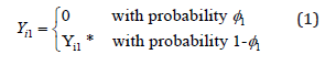
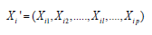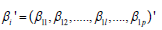Where Y_i1^* follows Poisson distribution with mean λ_1i with . In (1), represents the vector of P-dimensional covariates and represents the P-dimensional vector of regression parameters. The probability parameter 1 φ in (1) represents the proportion of excessive zeros in the count responses.

Based on assumption # 1, the probability mass function can be expressed as

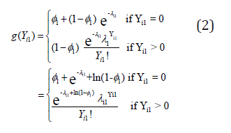
It can be shown that 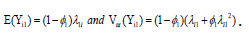If responses do not have any excessive zeroes (i.e. 1 φ = 0), then the probability mass function 1 ( ) i g Y in (2) is simplified to a Poisson distribution with rate 1i λ .

Assumption #2: Given Y_i1 , let Y_i2 , the random variable for the count of the second variable resulting from the ith subject, have the following conditional distribution as

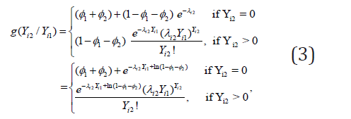
Where λ_i2 = exp(X′iβ₂) with X_i is as defined in (2) and β₂ = (β₂₁, β₂₂, . . . , β_2l, . . . , β_2P)′ represents the P -dimensional vector of regression parameters on the response variable Y_i2.

The above expression in (3) is developed based on the fact that Y_i2 will have three different categories. This is because as Y_i1 = 0 with probability ϕ₁, then Y_i2 has to be 0 with probability ϕ₁ as well. If Y_i1 > 0 , then Y_i2 still can be 0 with probability ϕ₂ or Poisson distribution with mean λ_i2Y_i1 with probability 1-ϕ₁−ϕ₂. Note that similar to Assumption 1, if the responses do not have excessive zeros (i.e. ϕ₁=0 and ϕ₂=0), then the conditional mass function in (3) reduces to a Poisson distribution with parameter λ_i2Y_i1. Thus, the bivariate joint mass function can be achieved by multiplying the marginal and conditional mass function derived in (2) and (3). Therefore, the bivariate mass function for Y_i1 and Y_i2 can be expressed as

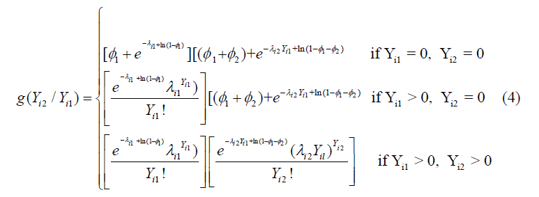
Under the assumption that the data do not have excessive zeros (i.e. φ₁= 0 and φ₂ = 0), the bivariate mass function in (4) will be simplied to the regular bivariate Poisson mass function which can be written as the bivariate exponential form

The bivariate zero-inflated Poisson mass function derived in (4) will be used to develop the likelihood function based estimating equation to estimate the model parameters.

Parameter estimation

In this section we present the estimation techniques of the model parameters based on likelihood approach. The likelihood function for the bivariate zero inflated Poisson model can be expressed as

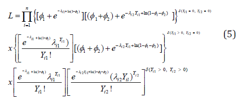
Where 1 2 ( , ) i i δ Y Y is the delta function which is equal to 1 if the condition inside the parenthesis is simplified or 0 otherwise. To estimate the regression parameters, we use the likelihood estimating equation which was derived by taking the _rst derivative of the logarithm of the likelihood function (5) with respect to the parameters. The 2(P+1)- dimensional vector of likelihood estimating equations can be simplified as

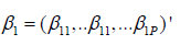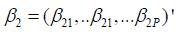In (6) are the P-dimensional vectors of the likelihood estimating equations which can be achieved by differentiating the logarithm of the likelihood function (5) with respect to and respectively. The explicit expressions of The explicit expressions of 1 11 ψ (β ) and 2 21 ψ (β ) are

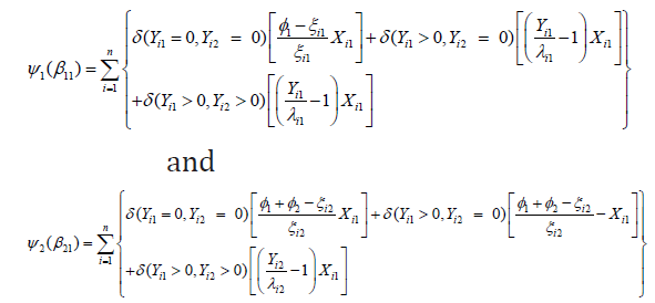
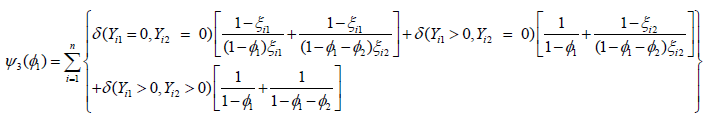
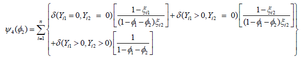
Respectively, where Similarly, ψ₃(φ₁) and ψ₄ (φ₂) can be obtained by differentiating the log-likelihood function with respect to φ₁ and φ₂ respectively, which has the following simplified form as

And

The estimates of the regression parameter vectors β₁ and β₂ and the probability parameters φ₁ and φ₂ can be found iteratively by using the following equation

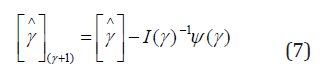
where denotes that the expression within the square brackets is evaluated at the r^th  iteration with 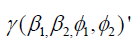Estimates of φ₁ φ₂ and can be obtained from the logit information of the bivariate count responses vectors of Y₁ and Y₂ respectively. To be specific, the estimate of φ₁ can be obtained from the response vector Y₁ sing the logit function (logit of P(Y₁=0)) of 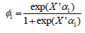where X is the covariate matrix and α is the corresponding vector of the parameters Albert et al. & Long et al. [23,24]. Similarly, the estimate of ϕ₂ can be obtained from the response vector Y₂ as logit of P(Y₂=0). It is noteworthy to point out that in the proposed bivariate Poisson-Poisson model we only require the estimates of  and rom the logit model. Thus, in the next section we will use the estimates of φ₁ and φ₂

The explicit expression of the 2(P+1)×2(P+1)-dimensional information matrix in (7), is presented in the Appendix. Note that the variance-covariance matrix of the regression parameters can be calculated by taking the inverse of the information matrix in (7). This estimation techniques presented in this section are used in next section to analyze the traffic accidents data [25-30].

In this section we apply the proposed methodology to the Virginia traffic accidents and Groningen traffic accidents data.

Virginia traffic accidents data

In this section, we apply the proposed zero-inflated Poisson-Poisson model to the Virginia traffic accidents data Leiter & Hamdan [11]. In this data set, daily counts of accidents and corresponding fatalities were investigated by Virginia Police Department for 639 days between January 1969 and October 1970. As the number of fatalities in a given day depends on the number of accidents, we assume that the number of accidents (Y₁) and the number of fatalities (Y₂) follows bivariate Poisson distribution. One major concern of modelling such bivariate Poisson responses is that the data may suffer the presence of excessive zeros. For example, there may be many days with no accident occurs, thus resulting the responses to be 0. Similarly, if there is no accident then there will be no fatalities. On the other hand, there may be many accidents without any fatalities. Consequently, both responses, the number of accidents (Y₁) and the number of fatalities (Y₂) may be zero-innated. Thus, one needs to incorporate zero-inflated while modelling such bivariate count responses. The summary table of the Virginia traffic accident is data presented in Table 1.

Table 1: Bivariate frequency distribution of number of accidents and fatalities for Virginia traffic accidents data.

Table 2: Effects of risk factors on Virginia traffic accident data under proposed bivariate zero- Inflated Poisson- Poisson model and bivariate Poisson-Poisson model without zero-inflation.

^aZero-inflated bivariate Poisson-Poisson regression model. ^bBivariate Poisson-Poisson regression model without zero-inflation.

We now use the proposed zero-inflated bivariate Poisson-Poisson model for analyzing Virginia Traffic accident data. In this data set we have only one covariate Year, which is a dummy variable with 0 if the year is 1969 and 1 if the year is 1970. We analyze the data using the zero-inflated bivariate Poisson-Poisson model (Model I) and bivariate Poisson-Poisson model without zero-inflated (Model II) and the results are presented in Table 2.

Table 2 indicates that there is no significant difference between the numbers of accidents occurs in year 1969 and 1970 under both models. Our results also indicate that the estimates of  the probability of no accident, is 0.4476. The probability of fatalities, under the condition that there are at least one accident appear to be 0.4976.

Groningen traffic accidents data

Our proposed model is also illustrated to accidents and fatalities data recorded in the city of Groningen, The Netherlands. The data were obtained from the database BRON of the Ministry of Transport, The Netherlands and presented in Table 3 of Meintanis [9]. In particular, we have the total accidents and fatalities recorded on Sundays of each month over the period between January 1997 and December 2004 in Groningen, The Netherlands. As the number of fatalities in a given month depends on the number of accidents, we assume that the monthly number of accidents (Y₁) and the number of fatalities (Y₂) due to those accidents follow a bivariate Poisson distribution. Similar to the Virginia traffic accident data, we now use the proposed zero-inflated bivariate Poisson-Poisson model for analyzing Groningen traffic accident data.

To do that we consider Time and Quarter as covariates. As we have accident and fatality records of 96 months, we consider Time = 1 for January 1997, Time=2 for February 1997 … and Time = 96 for December 2004. We use logarithm of time, log(Time), as a covariate in the data analysis. The covariate Quarter was constructed by considering Quarters 1, 2, 3 and 4 as between January-March, April-June, July-September and October-December, respectively. As we have 4 categories in the covariate Quarter, we have considered three dummy variables in our analysis Quarter 2, Quarter 3 and Quarter 4 assuming Quarter 1 as the base category. It is noteworthy to point out that as in the data set monthly records of accidents were recorded, it appears that the first response variable Y₁ does not have any zero responses. Thus, we assume the probability of excessive zeros, is zero to analyze Groningen traffic accidents data. Our analysis results are presented in Table 3.

Table 3 indicates that the effects of Time and various Quarters on number of accidents are similar under the proposed zero-inflated model (Model I) and the model without zero- inflation (Model 2). This is because as the number of traffic accidents (Y₁) does not have any excessive zeros, the proposed zero-inflated model has behaved like the regular bivariate model. Our results in Table 3 indicates that the covariate log(Time) has negative significant effect on numbers of accidents. That means as the time increases, the numbers of accidents decreases.

Table 3: Effects of risk factors on Groningen traffic accident data under proposed bivariate zero-Inflated Poisson- Poisson model and bivariate Poisson-Poisson model without zero-inflation.

^aZero-inflated bivariate Poisson-Poisson regression model. ^bBivariate Poisson-Poisson regression model without zero-inflation.

This is probably natural as new road safety rules appear to be implemented every year to reduce the risk of accidents. Our results also indicate that the numbers of accidents are significantly higher in Quarters 2, 3 and 4 as compared to Quarter 1. This is probably because the driving activities in the other quarters are more as compared to Quarter 1 as Quarter 1 normally represents winter months including January and February be the coldest month of the year with only an average of 2 hours of sunshine every day in Groningen. Less traffic may naturally mean less traffic related accidents. Table 3 also indicates that given that at least one accident occurs, the number of fatalities is significantly lower for Quarters 2, 3 and 4 as compared to Quarter 1. This indicates that Quarter 1 has more fatalities as compared to other quarters although Quarter 1 has less traffic accidents. This is probably because although there may be less accidents in winter months (January-March) but the fatalities may be higher if accidents occur as accidents can be severe due to frost, poor visibility etc. during the winter months. Our results also indicate that given that at least one accident occurs, the number of fatalities increases as the time progresses. It is noteworthy to point out that new safety rules may reduce the number of accidents, but the number of fatalities can be increased based on severity of accidents.

In this section we have compared the analysis results of the proposed zero-inflated bi-variate Poisson- oisson model (Model I) and bivariate Poisson-Poisson model (Model II). The bivariate Poisson-Poisson model has marginal-conditional interpretations, as the bivariate marginal and conditional means of the count responses are linked to the covariates and corresponding regression parameters. It is noteworthy to point out that for the zero inflated bivariate Poisson-Poisson model, the overall mean of the count responses is smaller than the mean without the excess zero responses. This is because the overall mean under the zero-inflated model is the multiplication of the probability of non-excess zero responses and the mean of non-excess zero responses. Furthermore, in the zero-inflated model the covariate and the corresponding regression parameters are linked to the mean of the non-excess zero responses.

We propose a marginal-conditional approach based zeroinflated bivariate Poisson-Poisson model for analyzing zero-heavy bivariate count responses. Our proposed model was illustrated in two traffic accident data sets. In the traffic accident and fatalities data, the count response variables, number of accidents and number of fatalities are expected to be correlated resulting in a bivariate Poisson distribution. To analyze such bivariate data, we need to take into account the problem of excess zeros because many days and/or months may not have any occurrence of accidents and sometimes even if they have accidents, they may not any fatalities. At this backdrop, the problem of zero-inflation may distort the results obtained from the model assuming a bivariate Poisson regression model. In bivariate count data this problem poses a formidable difficulty to the users of bivariate count data in various fields of applications.

In this paper, a simple generalized linear zero-inflated model is proposed for bivariate count data using the marginal-conditional probabilities. The link functions are obtained for the bivariate zero-inflated Poisson model where the marginal probability of the number of accidents and the conditional probability of the variable on the number of fatalities for given values of the number of accidents are considered to follow the Pois- son distributions. The results indicate some notable changes both in the magnitude and direction of the estimates. Finally, the model is fitted and compared with the fitted model based on the bivariate Poisson generalized linear model. The proposed zero-inflated model shows improvement in the fitted of the model. It also displays that if the data set does not have excessive zeros, then the proposed model will likely produce the results of the bivariate Poisson models without zero-inflation. Although the proposed methodology was applied in two traffic accidents data but our approach can be generalized and utilized in the other areas of research as well.

In this section we present the structure of the 2(P+1)×2(P+1)- dimensional information matrices I (γ ) as

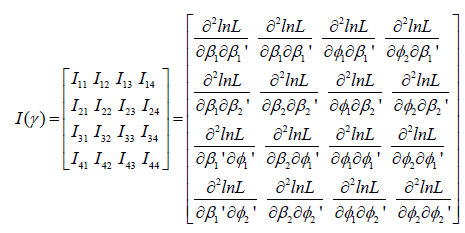
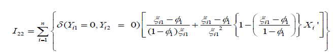
After some algebra, the explicit expression of (P+1)×(P+1)- dimensional matrix can be simplified as

Where is as defined in (6). Note that in I (γ ) matrix 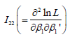is a (P+1) × (P+1) dimensional matrix with 0. Similarly, the (P+1) × 1-dimensional matrix of 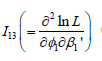can be simplified as

and 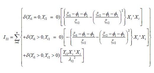is a (P+1)×1- dimensional matrix with 0.

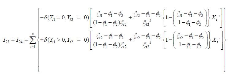
Using the derivation similar to the above, it can be shown that I₂₃ and I₂₄ are both (P+1)×1- dimensional matrices and have the following simplified form as

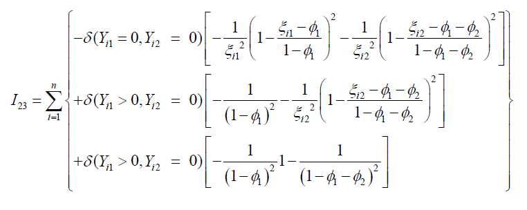
The explicit expression of the scalar quantities I₃₃ and I₃₄ , are

and

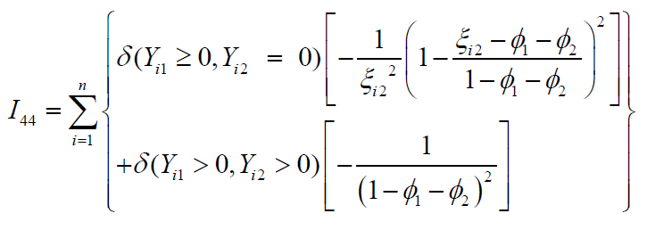
respectively. Finally, I₄₄ is also a scalar quantity which has the following simplified form as

Authors acknowledge gratefully that the study is supported by the HEQEP sub-project 3293, University Grants Commission of Bangladesh and the World Bank.

1. Long DL, Preisser JS, Herring AH, Golin CE (2015) A marginalized zero-inflated Poisson regression model with random effects. J R Stat Soc Ser C Appl Stat 64(5): 815-830.
2. Wang X, Chen MH, Kou RC, Dey DK (2015) Bayesian spatial-temporal modeling of ecological zero-inflated count data. Stat Sin 25(1): 189-204.
3. Arab A, Holan SH, Wikle CK, Wildhaber ML (2012) Semiparametric bivariate zero-inflated Poisson models with application to studies of abundance for multiple species. Environmetrics 23(2): 183-196.
4. Smith ANH, Anderson MJ, Millar RB, Willis TJ (2014) Effects of marine reserves in the context of spatial and temporal variation: an analysis using Bayesian zero-inflated mixed models. Marine Ecology Progress Series 499: 203-216.
5. Neelon B, Chang HH, Ling Q, Hastings NS (2016) Spatiotemporal hurdle models for zero-inflated count data: Exploring trends in emergency department visits. Stat Methods Med Res 25(6): 2558-2576.
6. Morgan CJ, Lenzenweger MF, Rubin DB, Levy DL (2014) A hierarchical finite mixture model that accommodates zero-inflated counts, non-independence, and heterogeneity. Stat Med 33(13): 2238-2250.
7. Kassahun W, Neyens T, Molenberghs G, Faes C, Verbeke G (2014) Marginalized multilevel hurdle and zero-inflated models for over dispersed and correlated count data with excess zeros. Statistics in Medicine 33(25): 4402-4419.
8. Papageorgiou H, Loukas S (1988) On estimating the parameters of a bivariate probability model applicable to traffic accidents. Biometrics 44(2): 495-504.
9. Meintanis SG (2007) A new goodness-of-fit test for certain bivariate distributions applicable to traffic accidents. Statistical Methodology 4(1): 22-34.
10. Lambert D (1992) Zero-inflated poisson regression, with an application to defects in manufacturing. Technometrics 34(1): 1-14.
11. Leiter RE, Hamdan MA (1973) Some bivariate probability models applicable to traffic accidents and fatalities. International Statistical Review 41(1): 87-100.
12. Karlis D, Ntzoufras I (2003) Analysis of sports data by using bivariate poisson models. Journal of the Royal Statistical Society D (The Statistician) 52(3): 381-393.
13. Jung R, Winkelmann R (1993) Two aspects of labor mobility: A bivariate poisson regression approach. Empirical Economics 18: 543-556.
14. Hofer V, Leitner J (2012) A bivariate Sarmanov regression model for count data with generalised Poisson marginals. Journal of Applied Statistics 39(12): 2599-2617.
15. Islam MA, Chowdhury RI (2015) A bivariate poisson model with covariate dependence. Bulletin of Calcutta Mathematical Society 107: 11-20.
16. Cacoullos T, Papageorgiou H (1980) On some bivariate probability models applicable to traffic accidents and fatalities. International Statistical Review 48(3): 345-356.
17. Cacoullos T, Papageorgiou H (1982) Bivariate negative binomial-Poisson and negative binomial-Bernoulli models with an application to accident data. In: Rao CR & Kallianpure G (Eds.), Statistics and Probability: Essays, North Holland, Amsterdam, Netherlands, pp. 155-168.
18. Holgate P (1964) Estimation for the bivariate poisson distribution. Biometrika 51: 241-245.
19. Consul PC (1989) Generalized poisson distributions: Properties and applications. Marcel Dekker, New York, USA.
20. Consul PC, Jain GC (1973) A generalization of the poisson distribution. Technometrics 15(4): 791-799.
21. Consul PC, Shoukri MM (1985) The generalized Poisson distribution when the sample mean is larger than the sample variance. Communications in Statistics-Simulation and Computation 14(3): 667-681.
22. Li CS, Lu JC, Park J, Kim K, Brinkley PA, et al. (1999) Multivariate zero-inflated poisson models and their applications. Technometrics 41: 29-38.
23. Albert JM, Wang W, Nelson S (2014) Estimating overall exposure effects for zero-inflated regression models with application to dental caries. Stat Methods Med Res 23(3): 257-278.
24. Long DL, Preisser JS, Herring AH, Golin CE (2014) A marginalized zero-inflated poisson regression model with overall exposure effects. Statistics in Medicine 33(29): 5151-5165.
25. Cheung YB, Lam KF (2006) Bivariate poisson-poisson model of zero-inflated absenteeism data. Stat Med 25(21): 3707-3717.
26. Consul PC (1994) Some bivariate families of lagrangian probability distributions. Communications in Statistics-Theory and Method 23(10): 2895-2906.
27. D´enes FV, Silveira LF, Beissinger SR (2015) Estimating abundance of unmarked animal populations: accounting for imperfect detection and other sources of zero inflation. Methods in Ecology and Evolution 6(5): 543-556.
28. Karlis D, Ntzoufras I (2005) Bivariate Poisson and diagonal inflated bivariate poisson regression models. R Journal of Statistical Software 14(10): 1-36.
29. Lee CT, Clark TT, Kollins SH, McClernon FJ, Fuemmeler BF (2015) Attention deficit hyperactivity disorder symptoms and smoking trajectories: Race and gender differences. Drug Alcohol Depend 148: 180-187.
30. Preisser JS, Stamm JW, Long DL, Kincade ME (2012) Review and recommendations for zero-inflated count regression modeling of dental caries indices in epidemiological studies. Caries Res 46(4): 413-423.