How Long Can an Ecological Model Predict?

Most fascinating in ecological systems is their complexity. Not only do ecological communities harbor a multitude of different species, even the interaction of just two individuals can be amazingly complex. For understanding ecological dynamics, this complexity poses a considerable challenge. In conventional mathematical models, the dynamics of a system of interacting species with considering the effect of omnivore on a small food web are described by a specific set of ordinary differential equations [1],

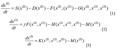
Here, [x⁽¹⁾, x⁽²⁾, x⁽³⁾] are the densities of prey, predator, and intraguild predator (i.e., top predator). S is the intrinsic gain by reproduction of the prey. F is the interaction between the predator and prey. G and H denote the loss of the resource and consumer from predation by the omnivore. K represents the gain of the omnivore that arises from this predation. [D, M, M] are the mortality, and γ is a constant conversion efficiency. Usually, S, F, G, H, and K are nonlinear functions. Equations (1) - (3) are treated as generalized ecological population model with revealing conditions for the stability of steady states in large classes of systems, identifying the bifurcations in which stability is lost, and providing some insights into the global dynamics of the system [1]. They can be seen as an intermediate approach that has many advantages of conventional equation-based models, while coming close to the efficiency of random matrix models.

It is widely recognized that the uncertainty in the generalized ecological population model (1) - (3) can be traced to three factors:

A. Observational errors [2],

B. Model errors such as uncertain model parameters [3-5], and

C. Chaotic dynamics [6-8]. Observational errors cause uncertainty in initial conditions. Discretization causes truncation errors. The chaotic dynamics caused by nonlinearity may trigger a subsequent amplification of small errors through a complex response.

A question arises: How long is the generalized ecological population model (1) - (3) valid since being integrated from its initial state? This has great practical significance. For example, if the model validity time shorter than the biological cycle, the model doesn’t have any capability to predict the biological cycle. In this paper, the first-passage time (FPT) is proposed to investigate ecological model predictability.

First passage time

The ecological model (1) - (3) can be generalized by a dynamical system. The state variables are usually defined by x(t) = [x⁽¹⁾(t), x⁽²⁾(t), x⁽³⁾(t)], a point in a three-dimensional phase space. Time evolution of x(t) from its initial condition x₀ is governed by the natural law

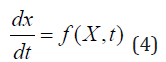
where f is a functional and X0 = X(t0). Let y(t) = [y⁽¹⁾(t), y⁽²⁾(t), y⁽³⁾ (t)] be the prediction point with an initial condition y(t₀ ) = y₀ y(t₀), and ε be the tolerance level for the prediction. The sprediction is valid if the state point x(t) is situated inside the ellipsoid ( S_ε , called tolerance ellipsoid) with center at y(t) and size ε . When y(t) coincides with x(t), the model has perfect prediction. The prediction is invalid if the state point x(t) touches the boundary of the tolerance ellipsoid at the first time from the initial state that is the first-passage time (FPT) for prediction [9,10] (Figure 1). FPT is a random variable when the model has stochastic forcing or initial condition has random error. Its statistics such as the probability density function, mean and variance can represent how long the model can predict. For simplicity and without loss of generality, a one-component population model is used for illustration.

Figure 1:Phase space trajectories of model prediction y (solid curve) and reality x (dashed curve) and error ellipsoid S_ε(t) centered at y. The positions of reality and prediction trajectories at time instance are denoted by “*” and “o”, respectively). A valid prediction is represented by a time period (t-t₀) at which the error first goes out of the ellipsoid S_ε(t).

One component population model

The simplest ecological model contains only one component. The model is based on the assumption that the population density has a maximum capacity K, the migration is proportional to the population density with the migration rate of m. The reproduction is carried out continuously by all its members, without regard to age or sex differences, at an average per capital rate r. The population density (ρ ) is normalized by K, 0 ≤ ρ ≤ 1. Usually, the model parameters r and m are difficult to measure. This may lead to the addition of stochastic forcing to the population model [1],

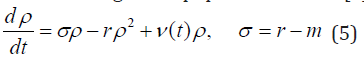
For simplicity, the stochastic forcing is assumed white multiplicative or additive noise,

where the bracket indicates the ensemble average; q represents the strength of the migration; and δ (t) is a delta function.

FPT Statistics

Let ρˆ(t) be the reference solution which satisfies (5) with the initial condition, 0 0 ρ (t ) = ρ . The forecast error ξ is determined as

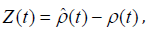
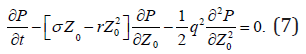
where ρ (t) is one of individual prediction corresponded to perturbing initial condition and /or stochastic forcing. The conditional probability density function (PDF) of the FPT (t-t₀) with a given initial error Z₀ satisfies the backward Fokker-Planck equation [11],

Integration of PDF over t leads to,

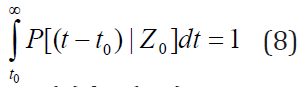
We multiply equation (7) by (t-t₀)n, integrate with respect to t from t₀ to ∞, use the condition (8), and obtain the equations of the nth moment of FPT

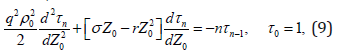
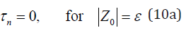
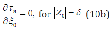
which is a linear, time-independent, and second-order differential equation with the initial error Z₀ as the only independent variable. If Z₀ =ε , the model has no predictability initially (i.e., the prediction point hits the error ellipsoid at t₀). FPT of prediction is zero, t − t₀ = 0 , which leads to the boundary conditions

If the initial error reaches the noise level (δ ), the boundary condition becomes [12],

Analytical solutions of (9) with the boundary conditions (10a, b) is

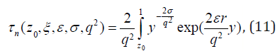
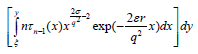
where τ₀ ≡1 , and z₀ ≡ Z₀/ε , ξ ≡δ /ε are non-dimensional initial error and noise level scaled by the tolerance level ε. The moments of FPT depend on two types of parameters:

A. Prediction parameters ( z₀ ,ξ ,ε ),

B. Model parameters (σ , r, q2).

Effects of prediction parameters

To investigate the dependence of mean FPT on the prediction parameters (z₀ ,ξ ,ε ) , the three model parameters are taken as r=1.0, σ =0.6, q2=0.2. Figure 2 shows the dependence of rτ₁(z₀ ,ξ ,ε ) [non-dimensional mean FPT scaled by the reproduction rate] on (z₀ ,ξ ) for four different values of ε(0.01, 0.1, 0.15, 0.2). Following features can be obtained:

Figure 2:Contour plots of rτ₁(z₀, ξ ,ε ) versus 0 (z ,ξ ) for four different values of ε(0.01, 0.1, 0.15, 0.2) using the general production model with model parameters r = 1, σ = 0.6, q² = 0.2. The contour plot covers the half domain due to 0 .

A. For given values of (z₀ ,ξ ) [i.e., the same location in the contour plots], the mean FPT increases with the tolerance level (ε).

B. For a given value of tolerance level (ε), the mean FPT is almost independent on the noise level ξ (contours are almost paralleling to the horizontal axis) when the initial error (ξ ) is much larger than the noise level (ξ ). The effect of the noise level (ξ ) on the mean FPT becomes evident only when the initial error ( z₀ ) is close to the noise level (ξ ).

C. For given values of (ε ,ξ ), the mean FPT decreases with increasing initial error Z₀.

Effect of model parameter σ

To investigate the sensitivity of mean FPT to the model parameter σ , the other model parameters are taken as q²=0.2, r=1.0. The model parameter σ takes values of 0.3, 0.5, and 0.7. Figure 3 shows the dependence of rτ₁ (z₀ ,ξ ,σ ) versus Z0 for two tolerance levels (ε = 0.1, 0.2), two noise levels (ξ = 0.1, 0.6), and three different values of σ (0.25, 0.5, and 1.0). It is found that the mean FPT decreases with increasing σ for all combinations of noise level (ξ = 0.1, 0.6) and tolerance level (ε = 0.1,0.2) , which indicates that increase of σ reduces the model valid period.

Figure 3:Dependence of rτ₁ (z₀,ξ ,q ) on the initial condition error z₀ for q² = 0.2, r= 1.0, and three different values of σ(0.4, 0.6, 0.8) using the general production model with two different values of ε (0.1, 0.2) and two different values of noise level ξ(0.1, 0.6).

Effect of stochastic forcing

To investigate the sensitivity of mean FPT to the strength of the stochastic forcing, q², the other model parameters are set as σ = 0.6, r = 1.0 . Figure 4 shows the dependence of rτ₁ (z₀, ξ ,q ) on z₀ for two tolerance levels (ε = 0.1, 0.2), two noise levels (ξ = 0.1, 0.6), and three different values of q² (0.1, 0.25, and 0.5) representing weak, normal, and strong stochastic forcing. Two regimes are found:

A. Mean FPT decreases with increasing q2 for large noise level (ξ = 0.6),

B. Mean FPT increases with increasing q2 for small noise level (ξ = 0.1).

Figure 4:Dependence of rτ₁ (z₀, ξ ,q ) on the initial condition error z₀ for σ = 0.6, r = 1.0, and three different values of q²(0.1, 0.2, 0.4) using the general production model with two different values of ε (0.1, 0.2) and two different values of noise level ξ (0.1, 0.6).

This indicates the existence of stabilizing and destabilizing regimes of the dynamical system depending on stochastic forcing. For a small noise level, the stochastic forcing stabilizes the dynamical system and increase the mean FPT. For a large noise level, the stochastic forcing destabilizes the dynamical system and decreases the mean FPT.

The limitation of ecological models’ predictability can be represented FPT-the time when the model error first exceeds the tolerance level. FPT is usually a random variable due to model uncertainty such as uncertain initial condition and model parameters. The probability density function of FPT satisfies the backward Fokker-Planck equation. A theoretical framework was developed in this study to determine various FPT moments, which satisfy time-independent second-order linear differential equations with given boundary conditions. This is a well-posed problem and the solutions are easily obtained. For the population model, the mean FPT decreases with increasing initial condition error, random noise, and model parameter; and increases slowly with increasing tolerance level. Both stabilizing and destabilizing regimes are found in the population model depending on stochastic forcing. For a small noise level, the stochastic forcing stabilizes the population model and increases the mean FPT. For a large noise level, the stochastic forcing destabilizes the population model and decreases the mean FPT.

The Office of Naval Research and the Naval Postgraduate School funded this research. The author thanks Mr. Chenwu Fan for computational assistance.

1. Clark CW (1985) Bioeconomic modelling and fisheries management. John Wiley & Sons, New York, USA, pp. 11-12.
2. Chu PC, Lu SH, Liu WT (1999) Uncertainty of the South China Sea prediction using NSCAT and NCEP winds during tropical storm Ernie 1996. Journal of Geophysical Research Oceans 104: 11273-11289.
3. Ivanov LM, Chu PC (2007) On stochastic stability of regional ocean models to finite-amplitude perturbations of initial conditions. Dynamics of Atmosphere and Oceans 43 (3-4): 199-225.
4. Ivanov LM, Chu PC (2007) On stochastic stability of regional ocean models with uncertainty in wind forcing. Nonlinear Processes in Geophysics 14: 655-670.
5. Galanis G, Emmanouil G, Chu PC, Kallos G (2009) A new methodology for the extension of the impact of data assimilation on ocean wave prediction. Ocean Dynamics 59(3): 523-535.
6. Chu PC, Ivanov LM, Margolina TM, Melnichenko OV (2002) Probabilistic stability of an atmospheric model to various amplitude perturbations. Journal of Atmospheric Sciences 59: 2860-2873.
7. Chu PC (1999) Two kinds of predictability in Lorenz system. Journal of the Atmospheric Sciences 56: 1427-1432.
8. Ivanov LM, Chu PC (2019) Estimation of turbulent diffusion coefficients from decomposition of Lagrangian trajectories. Ocean Modelling 137: 114-131.
9. Chu PC (2006) First-passage time for stability analysis of the Kaldor model. Chaos, Solitons and Fractals 27(5): 1355-1368.
10. Chu PC (2008) First passage time analysis for climate indices. Journal of Atmospheric and Oceanic Technology 25: 258-270.
11. Chu PC, Ivanov LM, Fan CW (2002) Backward Fokker-Planck equation for determining model valid prediction period. Journal of Geophysical Research Oceans 107(C6):
12. Chu PC, Ivanov LM (2005) Statistical characteristics of irreversible predictability time in regional ocean models. Nonlinear Processes in Geophysics 12: 129-138.