A Review of a Mathematical Model for a Direct Current Motor Using Control Analysis Methods

In this study, the simulation of control analysis examples with the software development have been created using Mathematica software, due to its strong symbolic language and the available tools it provides. The most commonly used analysis methods are simulated on separately excited DCM transfer functions. The simulations are created and modified as a small graphical area representing manipulation of the s-plane. The studied circuits have been used to analyze separately excited DCMs, which are shown in Figure 1, using a step response method and Bode diagrams, with and without a Proportional-Integral-Derivative (PID) controller [1-4].

Figure 1: Separately excited DCM standard schematic diagram.

The mathematical modeling of separately excited DCMs to obtain the transfer function between command input and output is shown in Figure 1. According to Figure 1 where Kirchhoff’s Voltage Law and mechanical equations are applied, the transfer function is derived as follows:

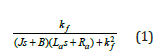
where k f is the motor constant, the armature coil is represented by an inductance and a resistance, is the friction coefficient and J (kg.m2 ) is the inertia torque. The control transfer function for a PID is shown in equation 2:

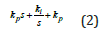
where kp ,kd ,ki are the proportional, derivative and integral gains respectively? Numerically, the rotor inertia value is J = 0.01 kg.m2 / s2 , the friction of the mechanical system, is B=0.1Nms/rad,, back emf and torque constant is k f = 0.01 Nm / A , the electrical circuit resistance is R a=1Ω , and the inductance is La = 0.5 H .

Equations (1) and (2) illustrate the step response and bode diagrams for the transfer function. Figure 2 correspond to the closed loop with control, the closed loop without control and the open loop transfer function, respectively, when unit step voltage is applied. In this way, the aim is to be able to explore how the locations of poles and zeros in the s-plane are affected by the step response.

Figure 2: Step response of DCM.

a. closed loop response without control and with control system,

b. open loop plot

The frequency response (Bode) diagrams below show the magnitude in dBs and the phase differences between the input and output. Adding a controller to the system changes the open-loop Bode plot, thereby changing the closed-loop response. With a given software service, students can check to see if the control meets the requirement specifications and can take part exercises provided by the lecturer. If so, the students are ready to move their project to the implementation and testing phases. The limit of angular frequency defines the horizontal axis obtained in the plot, and changes in the form of these limits are determined automatically by Mathematica. With these exercises users can easily integrate, improve and compare their knowledge. Some software program tools and commands are given in appendix. The Bode plots are given in detail with stability margins in Figure 3. The red-dashed line indicates the stability of the margins.

Figure 3: Bode Plots of transfer function open (a) and closed (b) and (c).

Using PID coefficients

kip=1.5; ki=2.5; kid=0.1.
pid=Transfer Function Model[(kip*s+ki+kid*s^2)/s,s];
input=Unit Step[t].
output=Output Response [closed Loop, input, t]; *)
dc motor [Kt_, Kf_,J_,B_,L_,R_]:=Transfer Function Model[ Kt/((J s+B )(L s+R)+Kt Kf ),s]
tmf=dc motor [0.02,0.02,0.015,0.001,0.005,1.3];
Close Loop=Systems Model Feedback Connect[tmf];
Open Loop=Systems Model Series Connect [Transfer Function Model[tmf], pid];
Closed Loop1=Systems Model Feedback Connect [open Loop];

Using tune activities

Open Loop1=PID Tune [tmf,”PID”,”PID Data”]

Gain and phase stability tools

Gain Phase Margins [Close Loop]
Gain Phase Margins [open Loop]
gpm=Gain Phase Margins[closedLoop1]
Gain Margins [Close Loop]
Phase Margins [Close Loop]
Map [{#[[1]], #[[1]]/Degree}&,%%%]

Bode plot

Bode Plot [tmf,{.01,100},Plot Label->”Bode Diagram- Open”, Label Style->Directive[Blue, Bold],Plot Style- {Directive [Thick, Color Data[20,1]],Directive[Thick, Color Data[20,9]]},Grid Lines>Automatic, Grid Lines Style Directive[Gray Level[0.9],Dashed],Stability Margins >True, Stability Margins Style{Green,Directive[Red, Dashed]}, Image Size >250,Frame >True,Plot Style {Directive[Thick, Color Data[20,1]],Directive [Thick,Color Data[20,9]]}, Frame >True, Frame Label {{“frequency(rad/s)”,”Magnitude(dB)”},{“frequency(rad/ s)”,”Phase(deg)”}},Plot Layout->”List”].

Bode Plot [Close Loop,{.01,100},Plot Label->”Bode Diagram Closed Loop without control”,Label Style-Directive[Blue, Bold],Plot Style {Directive[Thick, Color Data[20,1]],Directive[Thick,Color Data[20,9]]},GridLines >Automatic, Grid Lines Style Directive[GrayLevel[0.9],Dashed], Stability Margins >True, Stability Margins Style {Green, Directive[Red, Dashed]},Image Size >250,Frame >True, Plot Style {Directive[Thick, Col r Data [20,1]], Directive [Thick, Color Data[20,9]]},Frame >True, Frame Label {{“frequency(rad/s)”,”Magnitude(dB)”},{“frequency(rad/ s)”,”Phase(deg)”}},Plot Layout->”List”].

In this study, basic DCM analysis methods are shown for the control process of a DCM. Two different dynamic performance methods are presented with their features and then examined by using Mathematica software tools. It is thought that the study performed here is useful to control-related engineers and students to understand the effects of the analysis methods.

1. Fitzgerald C, Kingley S, Dumans S (2003) Electric, Machinery. (6^th edn), McGraw-Hill New York, USA.
2. Canizares CA, Faur ZT (1997) Advantages and disadvantages of using various computer tools in electrical engineering courses. IEEE Transactions on Education 40(3): 1-7.
3. Liebgott I (2016) Integration of the model-based design – industrial, approach - for teaching engineering science. IEEE Global Engineering Education Conference (EDUCON).
4. Wolfram Mathematica version 12.