
- About Us
- Information
-

The Author ensures that the research has been conducted responsibly and ethically with adherence to all relevant regulations. read more..
- For Authors
- For Reviewer
- Manuscript Guidelines
- Membership
- Publication Ethics
-
- Journals
- Reprints
- e-Books
- Videos
- Policies
- Contact Us
 COVID-19
- Submissions


Full Text
COJ Reviews & Research
Intelligent Cardiac Arrhythmia Identification System
Rahib H Abiyev*
Applied Artificial Intelligence Research Centre, Turkey
*Corresponding author: Rahib H Abiyev, Applied Artificial Intelligence Research Centre, Lefkosha, North Cyprus, Mersin 10, Turkey
Submission: December 10, 2018Published: December 19, 2018

ISSN: 2639-0590 Volume2 Issue1
Abstract
The design of an intelligent system for identification of cardiac arrhythmias is considered using ECG data set. The arrhythmia identification system that includes feature selection and classification stages is proposed. Cardiac arrhythmias are characterized by many input data. In the paper, a sequential feature selection method is used to reduce the size of the input feature space. The idea behind this study is to find out a reduced feature space so that a classifier built using this tiny dataset can perform better than a classifier built using the original dataset. After feature selection, fuzzy neural networks (FNNs) is applied for the classification purpose. The structure of FNNs is proposed and training algorithm is developed. The classification performance has been evaluated using 10-fold cross-validation. The proposed algorithms have been implemented and evaluated on the UCI ECG dataset. The proposed FNN based approach has provided attractive classification accuracy.
Keywords: Arrhythmia; Multivariate classification; Feature selection; Neural networks
Abbreviations: ECG: Electrocardiogram; SA: Sinoatrial; VFI5: Voting Feature Intervals; FE: Feature Elimination; ROC: Receiver Operating Characteristics; AUC: Area under the Curve; LVQ: Learning Vector Quantization; MSE: Mean Squared Error; SVM: Support Vector Machine; FNN: Fuzzy Neural Network; SFS: Sequential Feature Selection; FCM: Fuzzy C-Means Clustering; SFS: Sequential Forward Selection; SBS: Sequential Backward Selection
Introduction
This paper deal with cardiac arrhythmias to identify the heart diseases. Cardiac arrhythmia is also called abnormal rhythm and the problem appears in the rhythm of the heartbeat of the electrical activity of the heart which is irregular in beating or it’s beats become faster or slower than normal beats. Too fast heartbeat is called tachycardia (100 beats per minute or more) while too slow heartbeat is called bradycardia (60 beats per minute or less). Most arrhythmias are harmless, but some of them can be serious or even life-threatening that leads to death. The damage can happen to the brain, heart, or other organs when there is a lack of blood flow or heart may not be able to pump enough blood to the body [1].
Figure 1:Data flow diagram of an arrhythmia.

Electrical cardiac activity can be traced by ECG. The ECG waveform has key features which indicate sinus rhythm or arrhythmias (Figure 1). The 12 lead ECG has a standard form to recognize cardiac normality. The requirement of sinus rhythm of an electrocardiogram (ECG) to be classified as a normal sinus rhythm is: A heart rate (60-100) bpm; Regularity-Regular rhythm with less than 0.16 sec. variation in the shortest and longest duration between successive P waves; The sinoatrial (SA) node should pace the heart and P wave must appear in every QRS complex in a ratio of 1:1; PR interval is between 0.12 second and 0.20 second; QRS complex width should be less than 0.12 second.
Cardiac arrhythmia is a common type of heart disease that causes a heart attack. Coronary heart disease occurs when coronary arteries become narrowed because of building fat/cholesterol up within the artery wall. This causes imbalances and reduces flow blood and oxygen to the heart. There are many different types of cardiac arrhythmias. The atrial tachycardia is the rapid heartbeat, the atrial bradycardia is the slow one, and the irregular beat is known as atrial fibrillation and atrial flutter. The last one is common cardiac arrhythmia that leads to an irregular and sometimes rapid heart rate. These atrial arrhythmias may frustrate the heart’s ability to pump blood properly from its upper chambers (atria). The atria are not always empty completely when blood remaining there too long it stagnate and potentially clot. The clots may travel to other parts of the body, where they may cause blockages in the blood supply to the limbs, brain or heart [2]. The information obtained from an electrocardiogram (ECG) can be used to discover different types of heart disease, heart arrhythmia and heart attack. ECG device has twelve electrodes that measures the electrical activity of the heart (Figure 1). Every heartbeat generates 12 signals in ECG from a different angle that leads to gain many aspects of the electrical activity. Each of 12 leads has its own pattern. Generally, the descriptions of some indicators of the heart are given below.
a) QRS Complex: The QRS complex consists of the Q, R and S waves and represents ventricular depolarization. In some leads, some waves disappear like V1 does not contain a Q wave contain only an R wave and S wave still called QRS complex.
b) QRS interval: The normal duration of the QRS complex is 0.080 and 0.10 seconds And intermediate duration is 0.10 and 0.12 seconds. Abnormal QRS duration is greater than 0.12 seconds.
c) PR interval: Duration from the P wave to the starting of the QRS complex, it’s the time that electrical impulse generated in the sinus node to travel through the atria and across the AV node to the ventricles. The normal PR interval is 0.12 to 0.20 second.
d) QT interval: The QT interval is the time from the beginning of the QRS complex to the end of the T wave. The normal QT interval is less than 400-440ms.
e) T wave: The T wave followed QRS complex and it represents a ventricular repolarization. T waves in the right side in most leads (except aVR and V1).
f) P wave: The action potential of SA node that depolarizes the atria create P wave normally appears upright in lead 2. g) PR Interval: Duration from the start of the P wave to start of QRS complex, it represents electrical travelling from SA node to the AV node and to spread to ventricles, normally takes 0.12 to 0.20 seconds.
h) PR Segment: Duration from the end of the P wave to start of QRS complex.
i) Q Wave: Downward deflection, the first element in the QRS complex
j) RR interval: The duration between two sequence R waves.
k) ST interval: Duration from the end of S waves to the end of T wave.
l) ST segment: Duration from the end of S waves to the start of T wave.
A data gained from an electrocardiogram (ECG) is characterizing the electrical activity of the heart (cardiac). The information obtained from an electrocardiogram can be used to discover different types of cardiac arrhythmias. The aim of this study is to develop an intelligent system to classify arrhythmia ECG signals. Recently numbers of research works have been done for classification ECG signal. In these researches, the aim was the increase of the accuracy of the classification system. An original paper [3] uses VFI5 (Voting Feature Intervals) machine learning algorithm for the diagnosis of cardiac arrhythmia from standard 12 lead ECG Recordings. The VFI5 classification is based on a weight of voting among the classes. The classification made for each feature separately and the VFI5 algorithm achieved 62% accuracy. In [4], a kernel difference weighted k-nearest neighbors’ classifier (KDF-WKNN) is applied for the diagnosis of cardiac arrhythmia. In this paper, the cross-validation technique is applied to design the classification system [5]. represents feature elimination (FE) based ensembles learning method. The advantage of the proposed approach is the reduction of the size of feature space using various feature elimination methods.
The approach has provided an attractive performance in terms of overall classification accuracy. In [6] an automated artificial neural network-based classification system for cardiac arrhythmia using ECG recordings was presented. The classification performance is evaluated using six measures; classification accuracy, sensitivity, specificity, receiver operating characteristics (ROC), mean squared error (MSE) and area under the curve (AUC). The classification accuracy for test data was obtained as 86.67% [7]. Applied “learning vector quantization” (LVQ) neural networks for classification of arrhythmia dataset. LVQ create prototypes to define class boundaries. At first, the principal component analysis is used to reduce dimensionality then six LVQs are used for classification purpose. LVQ has shown better performance in reducing classification errors. In [8] Support Vector Machine (SVM) with Gaussian kernel had been used to classify the UCI ECG arrhythmias [9]. Uses feature extraction and classification methods for classification of ECG heartbeats into eight classes. Principal component analysis, linear discriminant analysis and probabilistic neural networks are used for these purposes [10]. Uses graph-based optimal path forest classifier method for detection of a cardiac arrhythmias. The system is tested using MIT BIH database. In [11] discrete wavelet transform is applied for feature extraction and multilayer neural networks for classification of cardiac arrhythmia. In [12] filter type feature selection is used to detect temporal, spectral and complex features. Hybrid classification method using SVM is applied for detection of cardiac arrhythmia [13]. Uses multilayer neural network that evolved particle be the approach for classification of cardiac arrhythmias using MIT BIH database.
Recently the fuzzy system and neural networks and also their integration are used for solving different classification problems [14-21]. These are classification of breast cancer [14,20], prostate cancer [15], erythemato-squamous diseases [16,19], liver disorders [17], Parkinson’s diseases [18], myocardial infarction [21], chest diseases [22]. The integration of neural networks and fuzzy systems are called fuzzy
neural networks or neuro-fuzzy system. The most clustering systems based on fuzzy neural networks [23,24] have two classes. These research papers demonstrate that the application of artificial intelligence methods for classification of various diseases and increasing recognition accuracy of the designed models become one of an important problem in computer science. In this paper multi-input and multi-output structure of FNN for classification of cardiac arrhythmias is presented.
The paper is organized as follows. Chapter 2 presents the design of the FNN’s structure for classification
cardiac arrhythmias. Chapter 3 describes the feature selection system used in the paper. Chapter 4 presents the techniques used in classification of arrhythmia ECG signals. The design algorithm of the proposed FNN is presented. Chapter 5 presents the parameter update algorithms. The used classification and gradient descent algorithms are presented. Section 6 presents simulation results. Finally, section 7 gives conclusions of the paper.
Cardiac Arrhythmia Classification System
The design of the intelligent system is divided into two levels: First is a feature selection that select best
feature from data using feature selection algorithms and the second level is a classifier with a fuzzy neural
Figure 2:Data flow diagram of an arrhythmia classification system.

network (FNN). The general conceptual structure of the system is given in (Figure 2). The first step is the filtering of ECG dataset samples from missing value. After filtering the data are scaled. This process helps the learning process of the system. As mentioned above arrhythmia dataset has characterized by many input parameters (features). Sometimes the collecting of these data and diagnosing the cardiac arrhythmia become too difficult. Less more important features are required to make an accurate decision.
In the paper, the feature selection algorithm is applied in order to select more important features of the arrhythmias. For this purpose, the sequential feature selection (SFS) algorithm is applied. The selected features are used for training of the classification system. After feature selection, the FNN is applied for classification purpose. In the training process, two cross-validation methods are used for the synthesis of the classification system: 10-fold crossvalidation and repeated random sub-sampling validation. After training the designed models are used for classification of cardiac arrhythmias in online mode.
In machine learning field the feature selection is sometimes known as attribute selection or feature subset
selection. Feature selection is an operation or process for selecting a subset of relevant features that are used in model construction. The basic expectation for using feature selection techniques is that the data contains many unusual data known as redundant or irrelevant features data. Redundant features mean that data which produce no more information than the currently selected features, and irrelevant features means that the data that produce unusual information. Feature selection techniques are a subset of the more common field of feature extraction. Feature selection keeps variable value, unlike feature extraction which generates new features value different from original features when the feature selection returns just a subset of the features. There are three main benefits feature selection techniques when constructing predictive models: Improved model accuracy, shorter times to create classifier (train model), avoid or reducing overfitting.
Sequential Feature Selection
Feature selection is used to reduce the data dimensions by selecting only a subset of measured features
for creating a model or classifier. Selection criteria generally include the minimization of a specific measure of classification error for models fit different subsets. Search algorithms are responsible to find an optimal subset of features for the classifier. Here the aim is to find and eliminate the unusual and irrelevant features and the size of the subset.
Feature selection is more desirable to feature transformation when the original units’ values are important, and the goal is to find an effective model for the chosen subset. In the case that feature was categorical then numerical transformations are inappropriate, therefore the feature selection becomes the primary of dimension reduction. Wrapper approaches consider the machine learning as a process in order to select subsets of features on the basis of their classification power. The basic idea of a wrapper approach is to deal with the classification accuracy of a specific machine learning algorithm in order to evaluate and perform the effectiveness of the selected subset of features. This approach was given by Kohavi &John [25]. A basic component of the wrapper approach is shown in (Figure 3). Wrapper method is too computationally and expensive but is simple. If the number of features is too large, then the execution time becomes long, and the exhaustive search becomes too expensive. The database used has k number of features, 2k possibility subsets need to be processed, in worst case 2k learning processes to run. In the paper, sequential feature selection is applied for feature reduction.
Figure 3:Diagram of Sequential feature selection.

Sequential feature selection components are
A. Classification function: known as a criterion, which is a method search to minimize over all feasible feature subsets. Criteria are misclassification rate. The objective function in this study is a classifier.
B. Greedy search strategies: it removes or adds features from a candidate subset while evaluating the criterion has been calculated. Sequential searches move in only one direction, always reducing or always growing the candidate set, and stopping criterion will be reached when all subset is all feasible feature subsets is created. If k is the number of features, the greedy search strategies needs, at maximum, k(k+1)/2.
Sequential search methods
There are two sequential search methods:
a) Sequential forward selection (SFS): the features are sequentially added to an empty candidate set until the addition of further features does not decrease the criterion.
b) Sequential backward selection (SBS): The features are sequentially removed from a full candidate set until the removal of further features increases the criterion.
Sequential Forward Selection is starting from the empty set, then add the feature sequentially (x*) when achieved highest results in the objective function J(Yk+X*). The features combined with the features (Yk)
that have already been selected. The objective function that used in this paper is a classifier which returns
misclassification rate. SFS algorithm is given in (Figure 4) [26].
1. Start with the empty set Y0 = {φ}
2. Select the next best feature 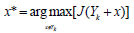
3. Update 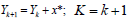
4.Go to step 2
Fuzzy Neural Network Based Classification
Building fuzzy neural network models from data involves methods based on fuzzy logic and neural networks. The model identification involves both structure and parameter estimation. The structure determines the flexibility of the model in the approximation of the unknown mappings. After the structure is fixed, the performance of a fuzzy model can be fine-tuned by adjusting the parameters. Turnable parameters are the parameters of the antecedent and consequent parts of the rules. In order to optimize the parameters, the training algorithms can be employed. Computational levels of an FNN’s model can be seen as a layered network structure [14].
The structure of the FNN model is constructed on the base of fuzzy rules. In the paper, the TSK-type IFTHEN fuzzy rules constructed by using linear functions are used. They have the following form.
If x1 is A1j and x2 is A2j and …and xm is Amj Then 
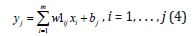
Here x1, x2,…,xm are input variables, yj (j=1,..,n) are output variables which are linear functions, Aij is a membership function for j-th rule of the i-th input defined as a Gaussian membership function. w1ij and bj (i=1,..m, j=1,…,r) are parameters of the network.
The fuzzy model that is described by IF-THEN rules can be obtained by modifying parameters of the conclusion and premise parts of the rules. In this paper, a gradient method is used to train the parameters of rules in the FNN structure.
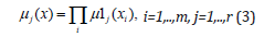
Using fuzzy rules in equation (1), the structure of the FNN is proposed (Figure 4). The FNN includes six layers. In the first layer, the number of nodes is equal to the number of input signals. These nodes are used for distributing input signals. In the second layer, each node corresponds to one linguistic term. For each input signal entering to the system, the membership degree to which input value belongs to a fuzzy set is calculated. To describe linguistic terms the Gaussian membership function is used.
Figure 4:Structure of FNN.

Here m is a number of input signals, r is a number of fuzzy rules (hidden neurons in the third layer). Cij and ij σ are centre and width of the Gaussian membership functions of the j-th term of i-th input variable, respectively. μ1j(xi) is the membership function of i-th input variable for j-th term.
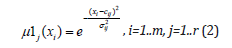
In the third layer, the number of nodes corresponds to the number of rules (R1, R2,…,Rr). Each node represents one fuzzy rule. To calculate the values of output signals, the product operation is used. In formula (3), Π is the min operation
The fourth layer is the consequent layer. It includes n linear functions that are denoted by LF1, LF2,…, LFn. The outputs of each linear function in Fig.1 are calculated by using the following equation (1-3).
In the fifth layer, the output signals of the third layer μ1(x )are multiplied with the output signals of nonlinear functions. In the sixth and seventh layers, defuzzification is made to calculate the outputs of the fuzzy neural networks.
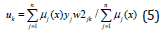
Here uk is the outputs of the sixth layer of the network. Here k=1,..,n.
After calculating the output signal of the FNN, the training of the network starts. Training includes the
adjustment of the parameter values of membership functions cij and σij (i=1,..,m, j=1,..,r) in the second
layer (premise part) and parameter values of linear functions w1ij, w2ij, bj (i=1,..,m, j=1,..,n) in the fourth
layer (consequent part).
Update of the parameters is implemented using fuzzy c-means clustering and gradient descent method.
Parameter Update
Fuzzy c‐means clustering
The design of FNN (Figure 1) includes the determination of the unknown parameters that are the parameters of the antecedent and the consequent parts of the fuzzy if-then rules (1). In the antecedent parts, the input space is divided into a set of fuzzy regions, and in the consequent parts, the system behavior in those regions is described. As mentioned above, recently a number of different approaches have been used for designing fuzzy if-then rules based on clustering [16,18,27,28], the least-squares method [28], gradient algorithms [14,17,20,24], genetic algorithms [28].
In this paper, the fuzzy clustering is applied to design the antecedent (premise) parts, and the gradient algorithm is applied to design the consequent parts of the fuzzy rules. Fuzzy clustering is an efficient technique for constructing the antecedent structures. The aim of clustering methods is to identify a certain
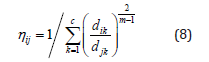
group of data from a large data set, such that a concise representation of the behavior of the system is produced. Each cluster center can be translated into a fuzzy rule for identifying the class. In this paper Fuzzy c-means clustering (FCM) is applied in order to partition the input data set and construct antecedent part of fuzzy if-then rules. Fuzzy c-means classification is based on the minimization of the following objective function [27]:
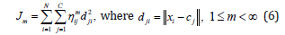
where m is any real number greater than 1, ηij is the degree of membership of xi in the cluster j, xi is the ith
of d-dimensional measured data, cj is the k-dimension centre of the cluster, and dij is any norm expressing
the similarity between any measured data and the centre [29].
Fuzzy partitioning is carried out through an iterative optimization of the objective function shown above,
with the update of membership ηij and the cluster centres cj. The algorithm is composed of the following
steps
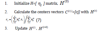
4. If {| H(t+1) − H(t ) |} <ε then stop; otherwise set t=t+1 and return to step 2.
After partition, each cluster center will correspond to the Centre of the membership function used in the input layer of FNN. The width of the membership function is determined using the distance between cluster
Centers [30-32].
Gradient descent
At first step, on the output of the network, the value of the error is calculated.
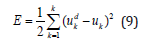
where K is a number of output signals of the network, dui and ui are the desired and current output values
of the network, respectively. The parameters w1ij, bj , w2jk (i=1,...,m, j=1,...,r, k=1,...,n) and cij and ij σ (i=1,..,m, j=1,..,r) are adjusted using the following formulas.
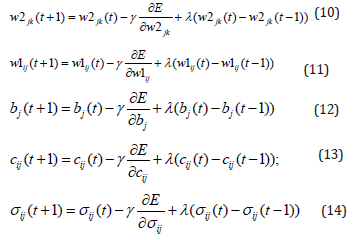
Here γ is the learning rate, λ is the momentum, m is a number of input signals of the network (input neurons) and n is the number of rules (hidden neurons). The values of derivatives in (10-12) are determined by the following formulas.
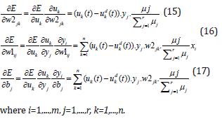
The derivatives in (13) and (14) are determined by the following formulas.
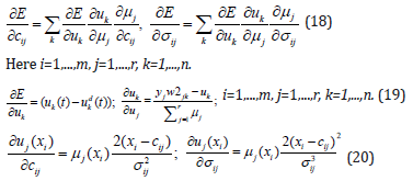
Using equations (18-20) in (13) and (14) the learning of the parameters of the FNN is carried out.
The whole training process includes the following steps:
a) The parameters of fuzzy neural networks are initialed in the interval of [0-1].
b) Fuzzy c means classification is applied to train data in order to determine the Centre and deviation of membership functions.
c) Input data are fed to FNN (forward propagation).
d) Outputs of the neurons of the hidden layer are computed (Feedforward process)
e) The outputs of the hidden layer are fed to the inputs of the output layer of FNN and the outputs of FNN are computed.
f) The error between current outputs and desired outputs (target) is computed.
g) The error is propagated back to the previous layer in order to update the weight coefficients of the neurons of the network. The backpropagation of error signal is continued until the update of all parameters in the layers is performed.
h) Repeating the steps 3 to 7 until the error becomes an acceptably small value.
Simulation
Table 1:Class description.

The arrhythmia dataset that was used in this paper was taken from the UCI Machine Learning Repository database. The database contains 13 classes with 452 samples and 279 features. From the 452 samples the 245 samples are normal and 207 arrhythmia instances. From 279 attributes the first four, age, sex, height, and weight, are the general description of the participant, and the other 276 attributes are extracted from the standard 12 lead ECG recordings. The following table (Table 1) shows the classes and the numbers of samples designated for each class [33,34].
The anthemia data was filtered and scaled. During filtration, the missed data and corresponding classes were cancelled. The classes having missing information are also cancelled. The final package of dataset after filtering contained 394 samples and 258 attributes, which represented 8 classes. After filtering, the values of the parameters are scaled in the interval 0-1. This process improves the learning of FNN parameters. As mentioned above the arrhythmia dataset has 258 inputs after filtering. This value is too large. In the paper, we apply a sequential feature selection algorithm in order to select more important features for classification purpose. Selecting the features is too computational and time-consuming and the number of features affects the time for computing the FNN’s output. But it is important to avoid overfitting and to create a classifier that will faster compute the output of the FNN. The dataset is divided into the train and test samples. The subset of selected features is generated using a greedy search strategy. The SFS feature selection algorithm with FNN classification is applied to select more important features. In the result of feature election, we have obtained 59 important features used for classification purpose.
For the classification purpose, we have applied two algorithmssupport vector machines and fuzzy neural networks. We used the recognition rate for the evaluation of the simulation results. At the first stage, we have used FNN for classification purpose. We have separated the data into training and testing sets. For this purpose, the k-fold cross-validation technique is applied.
FNN simulation through cross-validation
Cross-validation: Cross-validation is a model of validation technique for evaluating or estimating the results of a classifier. Cross-validation generalizes two independent data sets; training and testing. It is applied to find an accurate model of the classifier. There are many cross-validation techniques. In the paper two of them are using: K- fold cross-validation is used in the FNN model. In the k-fold cross-validation, the original data samples are randomly partitioned into k groups of equal size. A single subsample (group) is kept as a validation data for testing the model, and the remaining (k-1) subsamples are used as training dataset. The crossvalidation process is then repeated k times (number of folds). In each subsample, one set is used for validation and the remaining are used for training. The k number of results achieved from the folds and then are averaged in order to produce a single estimation (final classification accuracy). Repeated random sub-sampling validation technique randomly splits the dataset into training and validation data and repeated with a specific number of repeating. For each split, the model is fitted to the training data, and predictive accuracy is estimated using the validation data for every split. The results are then averaged over all the splits.
Classification: Fuzzy neural networks have been generated with initial random parameters. The 10-fold cross validation is applied to the data set for the training of FNN. In order to achieve high classification accuracy for the FNN based model, a set of experiments have been carried out using a different number of rules (number of neurons) in the hidden layer. The number of input neurons was 59, and the number of output neurons was 8 (number of classes). (Table 2) shows the results of experiments with a different number of hidden neurons (rules). The mean square error (MSE) is used to estimate the model performance. The goal value for MSE is taken as 0.05, the training has been performed for 6000 epochs. (Table 2) represents the simulation results of all FNN models with selected 59 features. (Table 3) represents the simulation results obtained with all (258) features.
Table 2:FNN with10-fold cross-validation with selected features (59 features).

The experiment number 5 in (Table 2) achieved (88.71) best accuracy with 65 neurons in a hidden layer. In Table 3, the experiment number 3 is achieved (79.39) best accuracy with 52 neurons in a hidden layer. These two tables show the different recognition accuracy with and without feature selection. As shown the selection of appropriate features allows improving the classification accuracy and decreasing the time for obtaining the final result. All experiments have been obtained with 10-fold cross-validation.
Table 3:FNN with10-fold cross validation without features selection (258 features).

(Table 4) shows a comparison of FNN based models with- and without feature selection using 65 hidden neurons (experiment 5 in Table 2 and Table 3). As shown the simulation results with feature selection mostly has good performance than without feature selection.
Table 4:FNN classification performance of arrhythmia data with and without feature selection for each class.

Table 5:SVM classification performance of arrhythmia data with and without feature selection for each class.

In the next stage, the simulation has been done using SVM with linear kernel was used in Matlab with LIBSVM library. The library helps quick creating of the classification model. Random sub-sampling validation was used in the training process. The results are used to evaluate classification accuracy. The number of random sub-sampling was (500), each one splits the data into 20% test and 80% train respectively. The two set of experiments were performed using with- and without feature selection. In the first experiment, the classification accuracy was obtained as 87.69% with feature selection (59 features), in the second experiment the classification accuracy was obtained as 85.18% without feature selection (258 features). As shown the selection of proper features allows improving the classification accuracy. (Table 5) shows class accuracy with and without feature selection. It has been noticed that most of the results of classes were improved with feature selection except class 2 and class 6. Compeering FNN based and SVM based models it becomes clear that they have shown nearly similar results with the little better performance of FNN.
The simulation results of FNN based- and SVM based models are compared with the results of other research works that have been used for classification of cardiac arrhythmias. (Table 6) demonstrates the comparisons of different models. As shown the results obtained using FNN based model with feature selection have better performance than other models.
Table 6:Comparative results of different models.

Conclusion
The paper presents cardiac arrhythmia identification system using fuzzy neural networks and support vector machine. The structure of the system is designed. The system includes feature selection and classification stages. The dataset of cardiac arrhythmia is taken from the UCI database, which was a good environment for testing the classifiers. The data is filtered, scaled and used for training of the classification system. By applying sequential feature selection algorithms 59 relevant features were selected and used for adjusting the parameters of classification systems based on FNN and SVM. The training is accomplished using k-fold cross-validation and repeated random sub-sampling validation. The results of training were evaluated using classification accuracy (or performance). FNN based classification was created with a different parameter. 10-fold cross-validation is used in training of FNN. The obtained results are averaged over 10 runs. The accuracy rate of FNN based model was obtained as 88.71% with feature selection, and 79.39% without feature selection. In the second stage, support vector machine classifier was tested. The repeated random sub-sampling is applied to the data. 500 random sub-sampling were created, each one split 80% train and 20% test data respectively. The accuracy rate was obtained as 87.69% with feature selection, and 85.18% without feature selection. It was shown that the use of sequential feature selection allows to improve the accuracy rate of the classifier. FNN has obtained good accuracy of 87.69% using feature selection.
References
- Hunter PJ, Pullan J, Smaill BH (2003) Modeling total heart function. Annual review of biomedical engineering 5(1): 147-177.
- Hampton J (2013) The ECG made easy. Elsevier Health Sciences, pp. 1-208.
- Altay Guvenir H, Burak A, Gulsen D, Ayhan C (1997) A supervised machine learning algorithm for arrhythmia analysis. In Proceedings of the Computers in Cardiology Conference, Lund, Sweden, pp. 433-436.
- Zuo WM, Lu WG, Wang KQ, Zhang H (2008) Diagnosis of cardiac arrhythmia using kernel difference weighted KNN classifier. In Proceedings of Computers in Cardiology, IEEE, pp. 253-256.
- Jadhav, Shivajirao, Sanjay N, Ashok G (2014) Feature elimination based random subspace ensembles learning for ECG arrhythmia diagnosis. Soft Computing 18(3): 579-587.
- Jadhav SM, Nalbalwar SL, Ashok Ghatol (2010) Artificial neural network based cardiac arrhythmia classification using ECG signal data. In Electronics and Information Engineering (ICEIE) IEEE International Conference on 1: 6-228.
- Alaa M (2009) Classification of ECG arrhythmia using learning vector quantization neural networks. In Computer Engineering & Systems ICCES. IEEE International Conference, pp. 139-144.
- Kohli N, Nishchal KV, Abhishek R (2010) SVM based methods for arrhythmia classification in ECG. In Computer and Communication Technology (ICCCT), IEEE International Conference, pp. 486-490
- Jeen Shing W, Wei Chun C, Ya Ting CY, Yu Liang H (2011) An effective ECG arrhythmia classification algorithm. Bio Inspired Comput Appl, pp. 545-550.
- José Da Luz ES, Nunes TM, Hugo De VC, Menotti D (2013) ECG arrhythmia classification based on optimum-path forest. J Expert Syst Appl Int J 40(9): 3561-3573.
- Sarkaleh MK, Shahbahrami A (2012) Classification of ECG arrhythmias using discrete wavelet transform and neural networks. Int J Comput Sci Eng Appl (IJCSEA) 2(1): 1-13.
- Alonso Atienza F, Morgado E, Fernández ML, García AA, Álvarez JL (2014) Detection of life-threatening arrhythmias using feature selection and support vector machine. IEEE Trans Biomed Eng 61(3): 832-840.
- Silvia Priscila S, Hemalatha M (2018) Diagnosis of heart disease with particle bee-neural network. Biomedical Research Special Issue: S40-S46.
- Rahib H Abiyev, Abdulkader Helwan (2018) Fuzzy neural networks for identification of breast cancer using images’ shape and texture features. Journal of Medical Imaging and Health Informatics 8(4): 817-825.
- Keles A, Hasiloglu A, Keles A, Aksoy Y (2007) Neuro-fuzzy classification of prostate cancer using NEFCLASS-J. Computers in Biology and Medicine 37(11): 1617-1628.
- Idoko JB, M Arslan M, Abiyev R (2018) Fuzzy neural system application to differential diagnosis of erythemato-squamous diseases. Cyprus Journal of Medical Sciences 3 (2): 90-97.
- Sallam M, Rahib Abiyev, Idoko JB (2017) Intelligent Classification of Liver Disorder Using Fuzzy Neural System. International Journal of Advanced Computer Science and Applications 8(12): 25-31.
- Abiyev R, Abizade S (2016) Diagnosing parkinson’s diseases using fuzzy neural system. Computational and Mathematical Methods in Medicine. Article ID 1267919, pp. 1-9.
- Idoko JB, Murat A, Abiyev R (2018) Intensive investigation in differential diagnosis of erythemato-squamous diseases. Cyprus Journal of Medical Sceinces 3: 90-97.
- Helwan A, Abiyev R (2016) Shape and texture features for identification of breast cancer. International Conference on Computational Biology, San Francisco, USA, pp. 19-21.
- Helwan A, Dilber UO, Abiyev R, John B (2017) One-year survival prediction of myocardial infarction. International Journal of Advanced Computer Science and Applications 8(6): 173-178.
- Abiyev R, Sallam M (2018) Deep convolutional neural networks for chest diseases detection. Journal of Healthcare Engineering, 2018: Article Number: 4168538, pp. 1-11.
- Abiyev R, Azad O, Boran S (2018) Detection of climate crashes using fuzzy neural networks. International Journal of Advanced Computer Science and Applications 9(2): 48-53.
- Abiyev R, Nurullah Aa, Ersin A, Günsel I, Çağman A (2016) Braincomputer interface for control of wheelchair using fuzzy neural networks. Biomed Research International, 2016: Article ID 9359868, pp. 1-9.
- Kohavi R, George J (1998) The wrapper approach. Feature Extraction, Construction and Selection, pp. 33-50.
- Isabelle G, André Elisseeff (2003) An introduction to variable and feature selection. The Journal of Machine Learning Research 3: 1157-1182.
- Bezdek JC (1981) Pattern recognition with fuzzy objective function algorithms. Plenum Press, New York, USA.
- Abiyev R (2011) Fuzzy wavelet neural network based on fuzzy clustering and gradient techniques for time series prediction. Neural Computing & Applications 20(2): 249-259.
- Uyar A, Fikret G (2007) Arrhythmia classification using serial fusion of support vector machines and logistic regression. Intelligent Data Acquisition and Advanced Computing Systems: Technology and Applications, IDAACS. 4th IEEE Workshop on, pp. 560-565.
- Kemal P, Şahan S, Güneş S (2006) A new method to medical diagnosis: Artificial immune recognition system (AIRS) with fuzzy weighted preprocessing and application to ECG arrhythmia. Expert Systems with Applications 31(2): 264-269.
- Thara S, Patrick B (2005) Classification of arrhythmia using machine learning techniques. WSEAS Transactions on computers 4(6): 548-552.
- Dayong G, Madden M, Chambers D, Gerard Lyons G (2005) Bayesian ANN classifier for ECG arrhythmia diagnostic system: A comparison study. Neural Networks IJCNN’05. Proceedings 2005 IEEE. IEEE International Joint Conference 4: 2383-2388.
- Aliferis CF, Tsamardinos I, Statnikov A (2003) HITON: A novel Markov Blanket algorithm for optimal variable selection. AMIA Annual Symposium Proceedings, pp. 21-25.
- Özçift A (2011) Random forests ensemble classifier trained with data resampling strategy to improve cardiac arrhythmia diagnosis. Computers in Biology and Medicine 41(5): 265-271.
© 2018 Rahib H Abiyev. This is an open access article distributed under the terms of the Creative Commons Attribution License , which permits unrestricted use, distribution, and build upon your work non-commercially.
Editor In Chief


.jpg)


Signup for Newsletter

Quick Links
 Editorial Board Registrations
 Submit your Article
 Refer a Friend
 Advertise With Us
Our Recent Edition

.jpg)


Top Editors


.jpg)


.bmp)
.jpg)
.png)
.jpg)


.jpg)


.png)

.png)


.png)


Financial Support

Sponsors

Latest e-Books

Latest Video

 a Creative Commons Attribution 4.0 International License. Based on a work at www.crimsonpublishers.com.
Best viewed in
a Creative Commons Attribution 4.0 International License. Based on a work at www.crimsonpublishers.com.
Best viewed in