Modeling and Reconstruction of Data in Signal Processing and Electronics

High-dimensional data interpolation in handwriting identification [1] is not only a pure mathematical problem but important task in pattern recognition and artificial intelligence such as: biometric recognition, personalized handwriting recognition [2-4], automatic forensic document examination [5,6], classification of ancient manuscripts [7]. Also, writer recognition [8] in monolingual handwritten texts is an extensive area of study and the methods independent from the language are well-seen [9-14]. Proposed method represents languageindependent and text-independent [15,16] approach because it identifies the author via a set of letters or symbols from the sample. Writer recognition methods in the recent years are going to various directions [17-19]: Texture analysis with Gabor filters and extracting features, using Hidden Markov Model [20] or Gaussian Mixture Model [21]. The paper wants to approach a problem of curve interpolation and shape modeling by characteristic points in handwriting identification [22]. Proposed method relies on nodes combination and functional modeling of curve points situated between the basic set of key points. Nowadays methods apply mainly polynomial functions, for example Bernstein polynomials in Bezier curves, splines [23] and NURBS. But Bezier curves don’t represent the interpolation method and cannot be used for example in signature and handwriting modeling with characteristic points (nodes). Numerical methods [24-26] for data interpolation are based on polynomial or trigonometric functions, for example Lagrange, Newton, Aitken and Hermite methods. These methods have some weak sides and are not sufficient for curve interpolation in the situations when the curve cannot be built by polynomials or trigonometric functions [27].

Multidimensional modeling of feature vectors

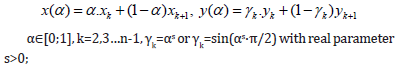
Proposed method has advancements over existing methods because it is computing (interpolating) unknown (unclear, noised or destroyed) values of features between two successive nodes (N-dimensional vectors of features) using hybridization of mathematical analysis and numerical methods, Calculated values (unknown or noised features such as coordinates, colors, textures or any coefficients of pixels, voxels and doxels or image parameters) are interpolated and parameterized for real number α_i∈[0;1] (i=1,2,…N-1) between two successive values of feature. This method uses the combinations of nodes (N-dimensional feature vectors) p₁=(x₁,y₁,…,z₁), p₂=(x₂,y₂,…,z₂),…, p_n=(x_n, y_n,…z_n) as h(p₁,p₂,…,p_m) and m=1,2,…n to interpolate unknown value of feature (for example y) for the rest of coordinates:

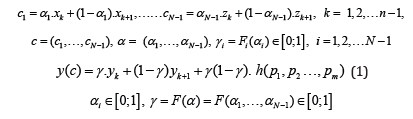
Then N-1 features c1,…, c_N-1 are parameterized by α1,…, α_N-1 between two nodes and the last feature (for example y) is interpolated via formula (1). Of course, there can be calculated x(c) or z(c) using (1). Two examples of h (when N=2) computed for MHR method [28] with good features because of orthogonal rows and columns at Hurwitz-Radon family of matrices:

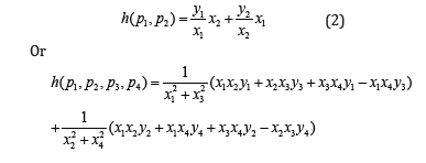
The simplest nodes combination is

and then there is a formula of interpolation:

Formula (1) gives the infinite number of calculations for unknown feature determined by choice of F and h. Nodes combination is the individual feature of each modeled data. Coefficient γ=F(α) and nodes combination h are key factors in data interpolation and object modeling.>

N-dimensional functions in modeling

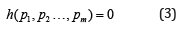
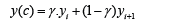
Unknown values of features, settled between the nodes, are computed using (1). Key question is dealing with coefficient γ. The simplest way of calculation means h=0 and γ_i=α_i. Then proposed method represents a linear interpolation. Each interpolation requires specific values of α_i and γ in (1) depends on parameters α_i∈[0;1]:

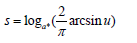
and F is strictly monotonic for each αi separately. Coefficient γi are calculated using appropriate function and choice of function is connected with initial requirements and data specifications. Different values of coefficients γ_i are connected with applied functions F_i(α_i). These functions γ_i=F_i(α_i) represent the examples of modeling functions for α_i∈[0;1] and real number s>0, i=1,2,…N-1. Each function is applied for different modelling:

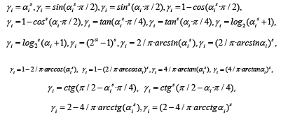
or any strictly monotonic function between points (0;0) and (1;1). For example, interpolations of function y=2x for N=2, h=0 and γ=αs with s=0.8 (Figure 1) is much better than linear interpolation. Functions γi are strictly monotonic for each variable α_i∈[0;1] as γ=F(α) is N-dimensional modeling function, for example:

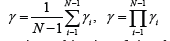
and every monotonic combination of γi such as

Figure 1:Two-dimensional modeling of function y=2^x with seven nodes and h=0, γ=α^0.8.

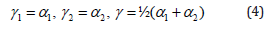
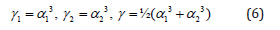
For example, when N=3 there is a bilinear interpolation:

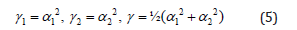
or a bi-quadratic interpolation:

or a bi-cubic interpolation:

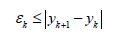
or others modeling functions γ. Choice of functions γ_i and value s depends on the specifications of feature vectors and individual requirements. What is very important: two data sets (for example a handwritten letter or signature) may have the same set of nodes (feature vectors: pixel coordinates, pressure, speed, angles) but different h or γ results in different interpolations (Figures 2-4). Here are three examples of reconstruction (Figures 2-4) for N=2 and four nodes: (-1.5;-1), (1.25;3.15), (4.4;6.8) and (8;7). Formula of the curve is not given. Algorithm of proposed retrieval, interpolation and modeling consists of five steps: first choice of nodes p_i (feature vectors), then choice of nodes combination h(p₁,p₂,…,p_m), choice of modeling function γ=F(α), determining values of α_i∈[0;1] and finally the computations (1). So, there are different data reconstructions with different modeling functions. As it can be observed, there is one extremum between two nodes for modeling with h≠0 (Figures 3&4). Comparing with polynomial or spline interpolations, there is one very important question: how to avoid extremum between each pair of nodes and how to minimize interpolation error? Generally current methods do not answer this key question. Nowadays methods of interpolations rely mainly on polynomials, especially on cubic splines. It means that there are interpolation polynomials W(x) of degree 3 for every range of two successive interpolation nodes (x_i,y_i) and (x_i+1, y_i+1). This method of cubic splines is C² class-this fact is very important in many applications of cubic interpolation. But second important feature of this method is interpolation error for function f(x):

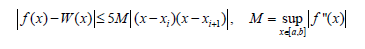
Figure 2:2D modeling for γ=α² and h=0.

Figure 3:2D reconstruction for γ=sin(α²·π/2) and h in [22].

Figure 4:2D interpolation for γ=tan(α²·π/4) and h=(x₂/x₁) + (y₂/y₁).

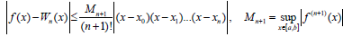
So, interpolation error depends on second derivative in the range of nodes [a;b] and this value cannot be estimated in general. Cubic spline can have extremum and may differ from interpolated function f(x) very much. Also, interpolation polynomial Wn(x) of degree n (Lagrange or Newton) for n+1 nodes (x₀, y₀), (x₁, y₁) … (x_n,y_n) is connected with unpredictable error in general with calculations of derivative rank n+1:

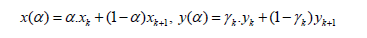
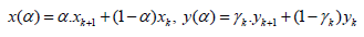
Proposed method with h=0 and α∈[0;1] represents formulas as convex combinations of nodes’ coordinates:

and interpolation error in general between two nodes looks as follows:

Proposed method is dealing with such significant features:
A. No extremum between two nodes.
B. Interpolation error does not depend on the value of derivative in the nodes or outside the nodes (even if derivative does not exist).
C. Interpolated function can be smooth in the nodes (class C¹).
D. Reconstruction of the function that much differs from the shape of polynomial, and not only function but any curve, also closed.
E. Extrapolation is calculated with the same formulas for α∉[0;1].
F. The idea of linear interpolation is applied for other modeling functions, not only γ=α¹.
G. Convexity between the nodes is fixed using two modeling functions:
γ_k=α_s or γ_k=sin(α^s·π/2) with real parameter s>0.

These two kinds of modeling functions are the simplest function, chosen via many calculations as follows:
a) γ_k=α^s if convexity is not changing between the nodes (x_k, y_k) and (x_k+1, y_k+1);
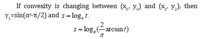
b) γk=sin(αs·π/2) if convexity is changing between the nodes (x_k, y_k) and (x_k+1, y_k+1).

Theorem if

A. There are given nodes of continuous function y=f(x): (x₀, y₀), (x₁, y₁) … (x_n, y_n), n≥2;
B. There are formulas to calculate values between the nodes:

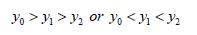
C. Three successive nodes are monotonic, for example let’s assume:

Then there is the method of 2D curve interpolation and extrapolation such as:
T.1: There is no extremum between two successive nodesinterpolated function is monotonic in the range of two nodes. T.2: Interpolated curve is class C⁰ (continuous) or C¹ (continuous and smooth).
T.3: Interpolation error does not depend on the value of derivative in the nodes or outside the nodes (even if derivative does not exist).
T.4: Convexity between two nodes (x_k, y_k) and (x_k+1, y_k+1) is fixed using modeling functions γ_k=α^s (if convexity is not changing) or γ_k=sin(α^s·π/2) (if convexity is changing).
T.5: Extrapolation is calculated with the same formulas for α∈[0;1].

Proof

T.1: Convex combination to calculate x(α) and y(α) between two nodes with strictly monotonic function γ_k gives us monotonic interpolation of the curve with no extremum between two nodes.

T.2: Interpolated curve is class C0 (continuous) just from definition of x(α) and y(α). Also, smooth interpolation between nodes is achieved with the same. Only smooth function in the inner nodes must be proved. Here is shown how to achieve smooth function in the inner nodes-let’s assume then y_k≠y_k+1 for each k. If y_k=y_k+1 for any k, then according to T.1 there must be the simplest linear interpolation between nodes (x_k, y_k) and (x_k+1, y_k+1) and interpolated curve is not smooth in nodes (x_k, y_k) and (x_k+1, y_k+1). For first three monotonic nodes (x₀, y₀), (x₁, y₁) and (x₂, y₂) there are calculations to fix parameter s for modeling function γ₁ between nodes (x₀, y₀) and (x₂, y₂) interpolating node (x₁, y₁) inside:

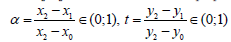
If convexity is not changing between (x₀, y₀) and (x₂, y₂), then γ₁=α^s and

A1 (beginning of the loop in algorithm for k=2,3…n-1): Having modeling function γ1 between nodes (x₀, y₀) and (x₂, y₂), it is possible for any α*→0 calculate

Then left difference quotient c is computed in the node (x₂, y₂):

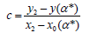
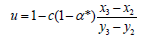
Of course, if value of derivative in (x₂, y₂) is known, c=f’(x₂)≠0. Then parameter u is fixed to obtain left (c) and right difference quotient equal in (x₂, y₂)-it means smooth in this node. If y₃ preserves the same monotonicity like y₂ and y1 (y₁>y₂>y₃ or y₁ < y₂< y₃) then

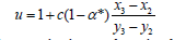
If y₃ does not preserve the same monotonicity like y₂ and y₁ then (because of different sign of left and right difference quotient0029

And as it was: if convexity is not changing between (x₂, y₂) and (x₃, y₃), then γ₂=α^s and

If convexity is changing between (x₂, y₂) and (x₃, y₃), then γ₂ = sin(α^s·π/2) and

So smooth interpolation function in the node (x₂, y₂) is achieved. And smooth interpolation for next range of nodes (x₃, y₃) and (x₄, y₄) is starting like loop A1 for k=3. And so on till last range of nodes (xn- 1, yn-1) and (x_n, y_n) for k=n-1 in A1.

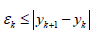
T.3: According to T.1 -interpolation error between two nodes for each k is equal:

T.4: These modeling functions are the simplest functions to achieve convexity changing or not.

T.5: Extrapolation left of first node (x₀, y₀) is done with modeling function γ₁ and α>1. Extrapolation right of last node (x_n, y_n) is done with modeling function γ_n-1 and α<0.

Then modeling function γ_n-1 must have domain with α<0. If not, there is possibility to define:

This theorem describes main features of proposed method.

The author’s method enables interpolation and modeling of high-dimensional data using features’ combinations and different coefficients γ: polynomial, sinusoidal, co sinusoidal, tangent, cotangent, logarithmic, exponential, arc sin, arc cos, arc tan, arc cot or power function. Functions for γ calculations are chosen individually at each data modeling and it is treated as N-dimensional function: γ depends on initial requirements and features’ specifications. Novel method leads to data interpolation as handwriting or signature identification and image retrieval via discrete set of feature vectors in N-dimensional feature space. So, this method makes possible the combination of two important problems: interpolation and modeling in a matter of image retrieval or writer identification. Main features of the method are: this interpolation develops a linear interpolation in multidimensional feature spaces into other functions as N-dimensional functions; nodes combination and coefficients γ are crucial in the process of data parameterization and interpolation: they are computed individually for a single feature; modeling of closed curves.

1. Marti UV, Bunke H (2002) The IAM-database: An English sentence database for offline handwriting recognition. Int J Doc Anal Recognit 5: 39-46.
2. Djeddi C, Souici Meslati L (2010) A texture-based approach for Arabic writer identification and verification. International Conference on Machine and Web Intelligence, Algeria, pp. 115-120.
3. Djeddi C, Souici Meslati L (2011) Artificial immune recognition system for Arabic writer identification. International Symposium on Innovation in Information and Communication Technology, Jordan, pp. 159-165.
4. Nosary A, Heutte L, Paquet T (2004) Unsupervised writer adaption applied to handwritten text recognition. Pattern Recogn Lett 37(2): 385-388.
5. Van EM, Vuurpijl L, Franke K, Schomaker L (2005) The Wanda measurement tool for forensic document examination. J Forensic Doc Exam 16: 103-118.
6. Schomaker L, Franke K, Bulacu M (2007) Using codebooks of fragmented connected-component contours in forensic and historic writer identification. Pattern Recogn Lett 28(6): 719-727.
7. Siddiqi I, Cloppet F, Vincent N (2009) Contour based features for the classification of ancient manuscripts. Conference of the International Graphonomics Society, pp. 226-229.
8. Garain U, Paquet T (2009) Off-line multi-script writer identification using AR coefficients. 10^th International Conference on Document Analysis and Recognition, Spain, pp. 991-995.
9. Bulacu M, Schomaker L, Brink A (2007) Text-independent writer identification and verification on off-line Arabic handwriting. International Conference on Document Analysis and Recognition, Brazil, pp. 769-773.
10. Ozaki M, Adachi Y, Ishii N (2006) Examination of effects of character size on accuracy of writer recognition by new local arc method. International Conference on Knowledge-Based Intelligent Information and Engineering Systems, Bournemouth, UK, pp. 1170-1175.
11. Chen J, Lopresti D, Kavallieratou E (2010) The impact of ruling lines on writer identification. 12^th International Conference on Frontiers in Handwriting Recognition, India, pp. 439-444.
12. Chen J, Cheng W, Lopresti D (2011) Using perturbed handwriting to support writer identification in the presence of severe data constraints. Document Recognition and Retrieval 7874: 1-10.
13. Chang S, Deng Y, Zhang Y, Zhao Q, Wang R, et al. (2022) An advanced scheme for range ambiguity suppression of spaceborne SAR based on blind source separation. IEEE Transactions on Geoscience and Remote Sensing 60: 1-12.
14. Chang S, Deng Y, Zhang Y, Wang R, Qiu J, et al. (2022) An advanced echo separation scheme for space-time waveform-encoding SAR based on digital beamforming and blind source separation. Remote Sensing 14(15): 3585.
15. Galloway MM (1975) Texture analysis using gray level run lengths. Comput Graphics Image Process 4(2): 172-179.
16. Siddiqi I, Vincent N (2010) Text independent writer recognition using redundant writing patterns with contour-based orientation and curvature features. Pattern Recogn Lett 43(11): 3853-3865.
17. Ghiasi G, Safabakhsh R (2013) Offline text-independent writer identification using codebook and efficient code extraction methods. Image and Vision Computing 31(5): 379-391.
18. Shahabinejad F, Rahmati M (2007) A new method for writer identification and verification based on Farsi/Arabic handwritten texts. Ninth International Conference on Document Analysis and Recognition, Brazil, pp. 829-833.
19. Schlapbach A, Bunke H (2007) A writer identification and verification system using HMM based recognizers. Pattern Anal Appl 10(1): 33-43.
20. Schlapbach A, Bunke H (2004) Using HMM based recognizers for writer identification and verification. 9th Int Workshop on Frontiers in Handwriting Recognition, Japan, pp. 167-172.
21. Schlapbach A, Bunke H (2006) Off-line writer identification using Gaussian mixture models. 18^th International Conference on Pattern Recognition, China, pp. 992-995.
22. Bulacu M, Schomaker L (2007) Text-independent writer identification and verification using textural and allographic features. IEEE Trans Pattern Anal Mach Intell 29(4): 701-717.
23. Schumaker LL (2007) Spline functions: Basic theory. (3^rd edn), Cambridge University Press, UK.
24. Collins GW (2003) Fundamental numerical methods and data analysis. Case Western Reserve University, USA.
25. Chapra SC, Canale RP (2012) Applied numerical methods. (7^th edn), McGraw-Hill, New York, USA.
26. Ralston A, Rabinowitz P (2001) A first course in numerical analysis. (2^nd edn), Dover Publications, New York, USA, p. 624.
27. Zhang D, Lu G (2004) Review of shape representation and description techniques. Pattern Recognition 1(37): 1-19.
28. Jakóbczak DJ (2014) 2D curve modeling via the method of probabilistic nodes combination-shape representation, object modeling and curve interpolation-extrapolation with the applications. LAP Lambert Academic Publishing, Saarbrucken, Germany, p. 88.