Modeling the Transmission Dynamics of LASSA Outbreaks in Nigeria States

This paper aimed at investigating LASSA through the dynamics of various factors that contribute in every stage of its transmission using a mathematical compartmental model based on data from the Nigerian states. LASSA Fever (LF) is an acute and sometimes severe viral hemorrhagic illness endemic in West Africa. The earliest cases of LASSA fever were thought to have occurred between 1920 and 1950, in Nigeria, Sierra Leone and Central African Republic and perhaps in other West African countries. However, the disease was first recognized in Nigeria in 1969, Ms. Lily (Penny) Pinneo (not real names), who was the first documented case of LF and from whom the first LASSA Fever Virus (LASV) was isolated in 1969. LASV is a single stranded RNA virus belonging to the Arenaviridae family of viruses. The virus is often named hemorrhagic fever virus because of the tendency to cause bleeding from body orifices. Sequencing of the small segment of the RNA of LASV has revealed the presence of four major lineages in West Africa with three in Nigeria (lineages I, II, and III) and one in the area comprising Ivory Coast, Sierra Leone, Liberia, and Guinea (lineage IV). Various viral strains have been associated with these major lineages with differences in their genome, serologic, and pathogenic characteristics. In Nigeria, mastomys natalensis have been identified by various names in some local languages including Eeku Asin (Yoruba), Jagba (Hausa), Nkapia or Nkakwu- (Igbo), and Isun (Kolokuma Ijaw) [1-10].

Infectious disease modelling

The central idea about transmission models, as opposed to statistical models, is a mechanistic description of the transmission of infection between two individuals. This mechanistic description makes it possible to describe the time evolution of an epidemic in mathematical terms and in this way connect the individual level process of transmission with a population level description of incidence and prevalence of an infectious disease. The rigorous mathematical way of formulating these dependencies leads to the necessity of analyzing all dynamic processes that contribute to disease transmission in much detail. Therefore, developing a mathematical model helps to focus thoughts on the essential processes involved in shaping the epidemiology of an infectious disease and to reveal the parameters that are most influential and amenable for control. Mathematical modeling is then also integrative in combining knowledge from very different disciplines like microbiology, social sciences, and clinical sciences. For many infections-such as influenza and smallpox-individuals can be categorized as either “susceptible,” “infected” or “recovered and immune.” The susceptible that are affected by an epidemic move through these stages of infection.

Compartmental models in epidemiology

Compartmental models are a technique used to simplify the mathematical modelling of infectious disease. The population is divided into compartments, with the assumption that every individual in the same compartment has the same characteristics. Its origin is in the early 20^th century, with an important early work being that of Kermack and McKendrick in 1927. The models are usually investigated through ordinary differential equations (which are deterministic), but can also be viewed in a stochastic framework, which is more realistic but also more complicated to analyze. Compartmental models may be used to predict properties of how a disease spreads, for example the prevalence (total number of infected) or the duration of an epidemic. Also, the model allows for understanding how different situations may affect the outcome of the epidemic, e.g., what the most efficient technique is for issuing a limited number of vaccines in a given population (Figure 1).

Figure 1: Common compartmental models in infectious disease modeling.

Framework for modeling for LASSA transmission dynamics

LASSA fever model presented in this study incorporates a model for the reservoir, which is Susceptible, exposed and infectious. This is done based on the assumption that susceptible rodent becomes exposed and then progress to infectious stage when they share unprotected storage of garbage, food stuff and water with infectious rodents or from inhalation of aerosols from urine and feces. These infected rats eventually tend to infect humans by direct contact or by inhalation of air follicles from dead infected rodents. It is also important to note that the existence of the exposed compartment is because of the incubation time that is the time it takes for an infected human to become infectious, which is twenty-one days for LASSA fever virus (Figure 2).

Figure 2: The SEIR model dynamics.

LASSA fever model presented in this study incorporates diagnostic factor, γ(ai)α1(ai)Eh(t,ai) (since early diagnostic enables treatment, that is 6 days after infection) and vaccination parameter (νh)which are critical for prediction and the need of extensions to enhance their predictive power for decision support; also a subdivision of rodent compartment called susceptible, exposed and infectious rodent with discrete age structure denoted by Sr(t,ej), Er(t,ej) and Ir(t,ej) respectively. This is done based on the assumption that susceptible rodent becomes exposed and then progress to infectious stage when they share unprotected storage of garbage, food stuff and water with infectious rodents or from inhalation of aerosols from urine and faeces [11-18].

Parameters

1. Recruitment term of humans Λ_h(ai)
2. Effective transmission rate in susceptible humans by infected rodents ρ(ai)
3. Effective transmission rate in susceptible humans by infected humans η(ai)
4. Treatment rate of exposed humans α₁(ai)
5. Treatment rate of infected humans α₂(ai)
6. Rate of inoculation κ(ai)
7. Progression rate of humans from the exposed state to the infectious state ε_h(ai)
8. Diagnostic factor of exposed humans γ(ai)
9. proportion of effective treatment of infected humans ψ(ai)
10. Natural death rate of humans µ_h(ai)
11. Progression rate of reservoirs from the exposed state to infectious state ε_r(ai)
12. Effective transmission rate in susceptible reservoirs by infected reservoirs β(ej)
13. Disease induced death rate of humans δ_h(ej)
14. Mortality of reservoirs due to hunting δ_r(ej)
15. Natural death rate reservoirs µ_r(ej)
16. Recruitment term of reservoirs Λ_r(ej)

We assume that the population is closed i.e. it is assumed that individuals who recovered from LASSA fever will never go back to susceptible class again (they remain recovered for life). The assumptions above suggest that LASV can only be transmitted from: (i) human to human (ii) rodent to human (iii) rodent to rodent, and as a result, we have the following schematic diagram and system of nonlinear ordinary differential equation (Figure 3).

Figure 3: Schematic diagram of transmission dynamics of Lassa fever

Figure 4: Multiple bar chart of the behavior of R0 in every state at varying intervention levels

Figure 4 explains the behavior of R0 at varying intervention levels, explained earlier in Table 3. This implies that at low intervention, Edo and Ondo has their R0 greater than 1, which implies instability in the states. This could be accounted for by the proximity between the two states (Edo state shares boundary with Ondo state). Furthermore, R0 is stable at both moderate intervention and high intervention in other states. This means that at moderate intervention, Lassa fever dies off gradually over a while.

Attached separately to keep the formatting intact

Formulating the Compartment into Differential Equation

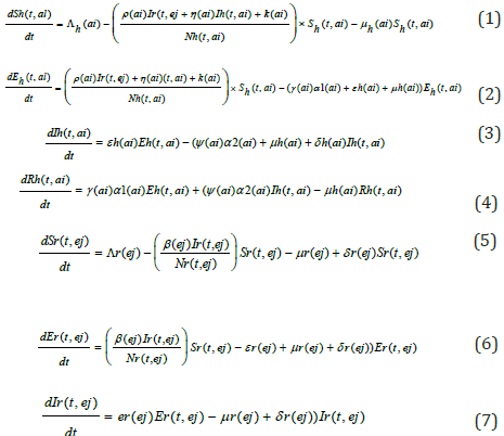
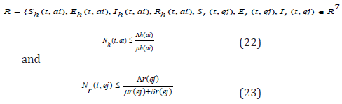
Since the formulated models monitor changes in the human and rodent populations; the parameters are assumed to ber nonnegative for all t ≥ 0, therefore the system of equations in (1) to (7) was analyzed within a feasible region R of biological interest. Theorem 1: The feasible region R defined by {Sh(t,ai),Eh(t,ai),Ih (t,ai),Rh (t,ai),Sr(t,ej),Er(t,ej),Ir(t,ej) ∈ R⁷ :

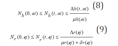
with initial conditions Sh(0,ai) ≥ 0,Eh(0,ai) ≥ 0,Ih(0,ai) ≥ 0,Rh(0,ai) ≥ 0,Sr(0,ej) ≥ 0,Er(0,ej) ≥ 0,Ir(0,ej) ≥ 0 is positive invariant for system (1) through (7).

Proof: If the total population size is given by

Nh(t, ai) = Sh(t, ai) + Eh(t, ai) + Ih(t, ai) + Rh(t, ai) and the total size of rodent population is

Nr(t, ej) = Sr(t, ej) + Er(t, ej) + Ir(t, ej)

Then one sees from (1) through (7) that

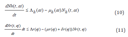
Considering the above equations as a linear differential we have that:

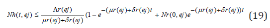
Solving the differential inequalities (8) and (9) one after the other gives

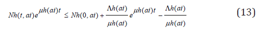
so that

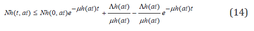
this implies

and

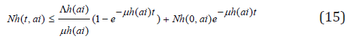
so that

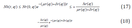
this implies

Taking the limits as t → ∞ gives

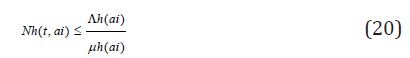
and

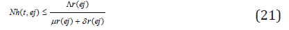
Thus, the following feasible region

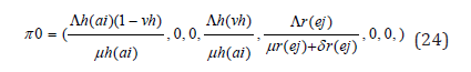
A disease-free equilibrium point is a steady-state solution where there is no LASSA fever infection. Solving the system of equation (3.1)-(3.7) in the absence of disease, we obtain the following equilibrium point,

We obtain a basic reproduction number R0 by expressing (1) to (7) as the difference between the rate of new infections in each infected compartment denoted by F and the rate of transfer between each infected compartment denoted by G

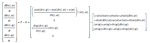
The Jacobian matrices J_F and J_G of F and G are found about π0 Where, T = J_FJ-1_G From the Jacobian matrices J_F and J_G of F and G found about π0, we have R₀, the maximum eigenvalue of T

Theorem 2: The disease-free equilibrium for the system (1) - (7) is locally asymptotically stable if R₀(ai)<1 and unstable if R₀(ai) >1. Proof:. The Jacobian of system (1) through (7) evaluated at the disease-free equilibrium point is

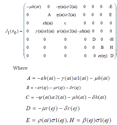
The first, fourth and fifth columns have diagonal entries, therefore the diagonal entries −µ_h(ai) twice and −µ_r(e_j) − δ_j (e_j) are three of the eigenvalues of the Jacobian matrix i.e λ1 =−µ_h(a_i), λ2 = −µ_h(a_i) and λ3 = −µ_r(e_j) − δ_r(e_j) . Thus, we find the remaining eigenvalues by excluding the corresponding columns and rows. The remaining eigenvalues are obtained from the submatrix

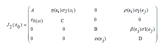
The eigenvalues of the matrix J₂(π₀) are the roots of the characteristic equation

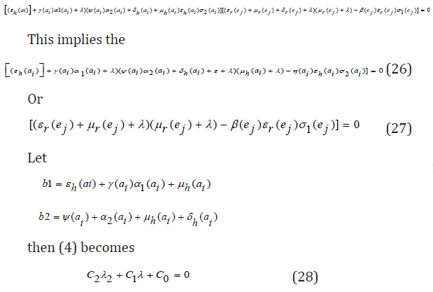
Further simplification of c ₀ in terms of R ₀(a) gives

C0 = b₁b₂ (1 − R₀ (a))

The Routh-Hurwitz criterion follows since all the roots of the polynomial (6) have negative real part if and only if the coefficient ci are positive and matrices Hi>0 for i = 0,1,2. From (7) it is shown that c₁>0 and c₂>0 since all b′ is are positive. Moreover, if R₀(a)<1 it is follows from (8) that c₀>0. All the eigenvalues of the Jacobian matrices J(π₀) have negative real part when R₀(a)<1 and the disease-free equilibrium point is locally asymptotically stable. However, when R₀(a)>1, we see that c₀<0 and by Descartes’ rule of signs ,there is exactly one sign change in the c₂,c₁,c₀ of coefficient of the polynomial (6). So, there is one eigenvalue with the positive real part and the disease-free equilibrium point is unstable. At this juncture, we can now infer from the equation (8) that there exists a c₀ such that and since R₀(a) majorizes R₀(a_i) the system (1) - (7) is locally asymptotically stable if R₀(ai)<1 and unstable if R₀(a_i)>1.

We shall use the theorem below to show that the developed model (1) - (7) has an endemic equilibrium point Ee. The endemic equilibrium point is a positive steady state solution when the disease persists in the population. Theorem 3: LASSA fever model (1) - (7) has no endemic equilibrium when R0(a)<1 and a unique endemic equilibrium exist when R0(a)>1.

Proof: Let Ee = (sh*, Eh*, Ih*, Rh*, Sr*, Er*, Ir*, ) be a non-trivial equilibrium of system (1) - (7) i.e. all component of Ee are positive. At the steady state, we get

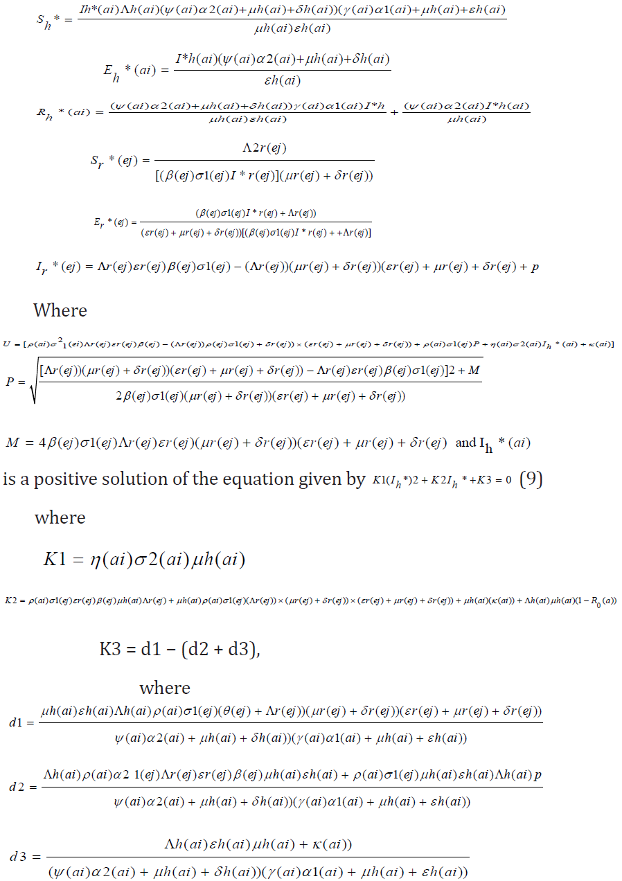
It is clearly seen that K₁>0. When R₀(a)<1 , one sees that K₂>0. However, when R₀(a)>1, then K₂<0 and endemic equilibrium exists. Finally, K₃<0 if d₁<(d₂ + d₃).

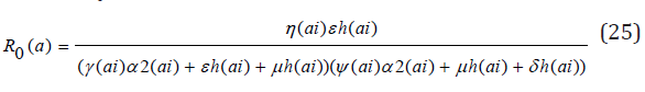
Sensitivity analysis is a statistical technique that can be applied to mathematical or computational models to provide insight on how uncertainty in the input variables affect the model outputs and which input variables tend to drive variation in the outputs. For models such as this infectious disease model, where the output is intended to inform decision-makers, uncertainty in the output can be disconcerting, as a single value is not given. However, the benefit is that a range of output values reveals a suite of possible model outcomes. It is sometimes of value to put in place robust policies that avoid the worst that can happen, although the policies may not achieve optimal results. If mitigating policies and alternatives are included and parameterized within the model, then sensitivity analysis can provide estimates of how responsive key output measures are with respect to these inputs. Sensitivity analysis tells us how important each parameter is to disease transmission. Such information is crucial not only for experimental design, but also to data assimilation and reduction of complex nonlinear models. Sensitivity analysis is commonly used to determine the robustness of model predictions to parameter values, since there are usually errors in data collection and presumed parameter values [19-24]. It is used to discover parameters that have a high impact on and should be targeted by intervention strategies. Sensitivity indices allow us to measure the relative change in a variable when a parameter changes. The normalized forward sensitivity index of a variable with respect to a parameter is the ratio of the relative change in the variable to the relative change in the parameter. When the variable is a differentiable function of the parameter, the sensitivity index may be alternatively defined using partial derivatives. Here, we present the sensitivity analysis of our Model using the formula given as

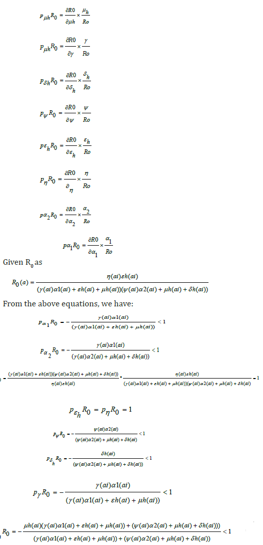
From the equations above, the most sensitive parameters are η(a₁) and ε_h which are Effective transmission rate in susceptible humans by infected humans and Progression rate of humans from the exposed state to the infectious state respectively. This implies that an increase or decrease in these parameters will cause an instability in R₀, as a result of its direct effect on R₀.

The data below was extracted from the National Center of Disease Control’s weekly Epidemiological Report on LF up till February 2019. Susceptible is the population of the state where LASSA fever has Incidence, Exposed is a percentage of the susceptible which is a function of effective transmission rate, Infected is a population reported confirmed, while death, is the death of confirmed cases (Figures 4-9); (Tables 1-4).

Figure 5: Multiple bar chart illustrating the behavior of R0 for every state at varying intervention levels.

Figure 6: Simple bar chart illustrating R0 at low intervention for every state at varying intervention levels.

Considering Figure 6 above, at low intervention, Lassa fever becomes epidemic at Edo and Ondo state, while the Ro is less than 1for other states which implies stability.

Figure 7: Simple bar chart illustrating R0 at moderate intervention for every state at varying intervention levels.

Considering Figure 7 above, at moderate intervention, Lassa fever becomes stable with the Ro is less than 1 for all states which implies stability.

Figure 8: Simple bar chart illustrating R0 at maximum intervention for every state at varying intervention levels.

Considering Figure 8 above, at high intervention, Lassa fever becomes stable with the Ro as low as 0.11 for all states which implies stability.

Figure 9: Case fatality of LASSA Across The Nigerian State.

Figure 9 explains case fatality as the percentage of those that are infected that eventually die. It is important to note that Kano, Rivers, Cross Rivers, Borno, Kwara, Benue, Imo, Abia and Adamawa, has 100% fatality with low case of incidence, while compared to states like Edo states,Ogun state, with higher cases of incedence have low case fatality. This could only be pointed to the factor of proximity to diagnostic centers, which exists only in three states in Nigeria. Literarily cases that occur in states closer to diagnostics centers gets fast intervention, as the disease can easily be diagnosed, and detected.

Figure 10: The distribution of confirmed Lassa fever cases in Nigeria.

Figure 10 above validates the first discovery that proximity to diagnostic center affect the case fatality of Lassa fever patient. Population of confirmed cases are more in Edo and Ondo state, which are closer to Lagos Diagnostic center, while places like Plateau, Bauchi, Gombe, are closer to irrua Diagnostic center at Jos.

Table 1: Extracted Data from the National Center of Disease Control (NCDC) and Susceptible is the population of the state where Lassa fever has Incidence, Exposed is a percentage of the susceptible which is a function of effective transmission rate, Infected is a population reported confirmed, while death, is the death of confirmed cases.

Table 2: Parameter structure used in the models and their sources and explains the values of parameters used in the estimation of R₀.

Table 3: Basic Reproduction number obtained across the state at three different levels of parameter and iterates the estimates of R₀ gotten from the data collected from NCDC and parameters in Table 2.

Table 4: Assumed Parameters of R0 at three different levels and above explains the varying degrees of interventions to reduce/stop Lassa fever which are captured by the above four parameters (Treatment rate of exposed humans α1(ai) Treatment rate of infected humans α2(ai), Diagnostic factor of exposed humans γ(ai) proportion of exective treatment of infected humans ψ(ai) )in all the compartments of the model. The values are varied at 0.1, which indicated little or no intervention, 0.5: which indicated medium intervention, while 0.9 indicates maximum intervention at these levels.

Considering the available data and the result of the sensitivity analysis, varying the values of four parameters which all signify effective and ineffective intervention, towards the eradication of the disease, showed a drastic reduction in R0, as the intervention level increased. It is also important to note that the lines with 100% fatality are states with first incidence of disease, especially places far away from diagnostic centers. This utmost depicts low diagnostics which is a function of proximity to test centers, which are in three places in Nigeria; National reference laboratory in Abuja, Lagos university teaching hospital (LUTH), Irrua specialist teaching hospital (ISTH), Institute of LASSA fever research and control (ILFRC), Irrua, Edo state, Nigeria.

The modification of the transmission dynamics between susceptible compartment to Exposed compartment by the removal of effective contact rate and interaction rate in reservoir has a positive effect on the R_0. At minimum intervention, Edo state and Ondo state has their R0>1 which implies instability. This means in time; LASSA fever will be epidemic in the two state. At mid intervention, R0<1 for all the states, which implies a steady state for the disease with minimal intervention. At maximum intervention R0 reduces to the barest below 0.2 in all states, which implies a steady state for the disease. Therefore, Proximity to diagnostic centers effective healthcare model has major part to play in eradicating LASSA fever in Nigeria.

1. Polyanin D, Manzhirov AV (2007) Mathematics for Engineers and Scientists, USA.
2. Safronetz D, Lopez JE, Sogoba, Traone SF, Raffel SJ, et al. (2010) Detection of Lassa virus. Mali Emerg Infect Dis 16(7): 1123-1126.
3. Dietz K, Heesterbeek JA (2000) Bernoulli was ahead of modern epidemiology. Nature 408(6812): 513-514.
4. Walker DH, Cormick JH, Johnson KM, Webb PB, Kombakano G, et al. (1982) Pathologic and virologic study of fatal Lassa fever in man. Am J Pathol 107(3): 349-356.
5. Eames KT, Keeling MJ (2003) Contact tracing and disease control. Proc Biol Sci 270(1533): 2565-2571.
6. Edmunds WJ, Medley GF, Nokes DJ (1999) Evaluating the cost-effectiveness of vaccination programmes: A dynamic perspective. Stat Med 18(23): 3263-3282.
7. Ferguson NM, Cummings DA, Fraser C, Cajka JC, Cooley PC, et al. (2006) Strategies for mitigating an influenza pandemic. Nature 442(7101): 448-452.
8. Ferguson NM, Keeling MJ, Edmunds WJ, Gani R, Grenfell BT, et al. (2003) Planning for smallpox outbreaks. Nature 425(6959): 681-685.
9. Grundmann H, Hellriegel B (2006) Mathematical modelling: a tool for hospital infection control. Lancet Infect Dis 6(1): 39-45.
10. Hadeler KP, Waldstatter R, Worz Busekros A (1988) Models for pair formation in bisexual populations. J Math Biol 26(6): 635-649.
11. Hale JK (1969) Ordinary differential equations. USA.
12. Hamer WH (1906) Epidemic disease in England the evidence of variability and persistency of type. Lancet 1: 733-739.
13. Hethcote HW, Yorke JA (1984) Gonorrhea transmission dynamics and control. USA.
14. Murray JD (2001) An introduction mathematical biology. USA.
15. James TO, Abdulrahman S, Akinyemi S, Akinwale NI (2005) Dynamics transmission of Lassa fever disease. International Journal of Innovation and Research in Education Sciences 2(1): 2349-5219.
16. Li MY, Mouldoney JS (1995) Global Stability for the SEIR model in epidemiology. Mathematical Biosciences 125(2): 155-164.
17. Mouldoney JS (1990) Compound matrices and ordinary differential equations, Rocky Mountain. Journal of Mathematics 20: 857-872.
18. Mccormick JB, Webb PA, Krebs JW, Johnson KM, Smith ES (1987) A prospective study of the epidemiology and ecology of lassa fever. Journal of Infectious Diseases 155: 437-444.
19. Onuorah MO, Akinwande NI, Nasir MO, Ojo MS (2016) Sensitivity analysis of Lassa fever model. International Journal of Mathematics and Statistic Studies 4: 30-49.
20. Ogbu OE, Ajuluchukwu CJ, Uneke CJ (2007) Lassa fever in West Africa sub-region: An overview. Journal of Vector Borne Diseases 44: 1-11.
21. Tomori O, Fabiyi A, Sorungbe A, Smith A, Cormick JB (1998) Viral hemorrhagic fever antibodies in Nigeria populations, Am J Trop Med Hyg 38(2): 407-410.
22. Okuonghae R, Okuonghae DA (2006) Mathematical model for Lassa fever. Journal of the Nigeria Association of the Mathematical Physics 10: 457-464.
23. Venden D, Watmough J (2002) Reproduction numbers and subthreshold endemic equilibria for compartment models of disease transmission. Math 180: 29-48.
24. Winn A, Walker (1975) The pathology of human Lassa fever, Bull. World Health Organ 52(4-6): 535-545.