
- About Us
- Information
-

The Author ensures that the research has been conducted responsibly and ethically with adherence to all relevant regulations. read more..
- For Authors
- For Reviewer
- Manuscript Guidelines
- Membership
- Publication Ethics
-
- Journals
- Reprints
- e-Books
- Videos
- Policies
- Contact Us
 COVID-19
- Submissions


Full Text
Aspects in Mining & Mineral Science
Chemical Potentials in Electrolyte Solutions
Grant Allakhverdov*
National Research Centre “Kurchatov’s Institute”, Moscow, Russia
*Corresponding author: Grant Allakhverdov, National Research Centre “Kurchatov’s Institute”, Moscow, Russia
Submission: March 01, 2022;Published: April 04, 2022

ISSN 2578-0255Volume9 Issue1
Abstract
Methods for calculating chemical potentials and activity of solution components are considered. It is shown that the standard state of chemical potentials in all cases is determined by the properties of a pure solvent. Examples of calculating the interphase distribution of components during crystallization from solutions are given.
Keywords: Free energy; Component activity; Chemical potential; Electrolyte solutions
Introduction
Chemical potentials play major role in the interphase distribution of components, due to the equality of their values in the coexisting equilibrium phases of the system. When comparing the distribution of various elements of multicomponent solutions, standardization and accuracy calculation of chemical potentials are of decisive importance, which is purpose of this article.
Theory
In statistical thermodynamics the main value has the determination of the chemical potential in the form
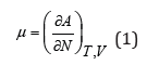
where A is the Helmholtz free energy, N is the number of particles, T is absolute temperature and V is the volume of system. The concept of component activity is related to the chemical potential
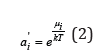
In this definition ai represented absolute activity [1]. In many cases, when comparing the properties of similar systems, the chemical potential can be represented as a function of relative activity ai, highlighting some component
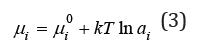
where 0iμ is the chemical potential in some common state for the compared systems, called the standard state, the choice of which is arbitrary. At the same time, this state should reflect the properties of the system under study
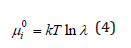
where λ is some constant parameter characterizing the state of the system at a given temperature. The free energy of the system can be determined using the equations of statistical thermodynamics as [1,2]
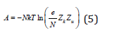
where e is the base of the natural logarithms, Zk, Zu are the partition functions associated with kinetic and potential energy respectively. The value Zk for gas systems, taking into account quantum effects, can be defined as [1,3]
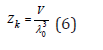
where 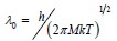 is the De Broglie heat wave, h is Plank’s
quantum constant, and M is the particle mass.
is the De Broglie heat wave, h is Plank’s
quantum constant, and M is the particle mass.
Combined Eq. (5) and (6), we have
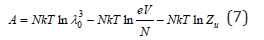
Differentiating Eq. (7) by volume, we can calculate the gas pressure
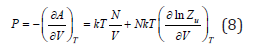
In the absence of interactions Zu=1, the gas called ideal, and the thermal equation of state (8) takes the form
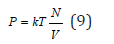
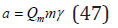
In the transition to solutions and considering the additive properties of thermodynamics potentials, the free energy of solution can be represented as

where Aw is the free energy of solvent, Zu is partition function that randomizes all types of interactions, including the interaction of solute particles N with solvent molecules Nw. The pressure of the solution, by analogy with Eq. (8), can be defined as
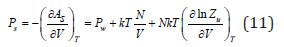
where the value of Pw refers to the pure solvent. Difference
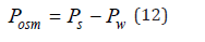
represents osmotic pressure. In dilute solutions at N≪Nw we can put Zu=1 and express the pressure of the ideal solution Pid as
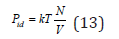
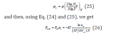
This is the Van’t Hoff equation, which has complete similarity to Eq. (9) and shows the acceptability of the general statistic model for gases and solutions [2,4]. The osmotic coefficient characterizing he degree of deviation from ideality, according to Eq. (12) and (13), can be defined as
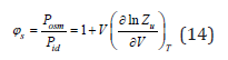
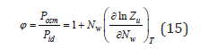
In the accepted approximation N≪Nw we can put it 0 V = Nwvw , where Nw and vw 0 are the number of solvent molecules and its molecular volume. In it is case osmotic coefficient can be determined as
and, accordingly Eq. (10), can be represented as
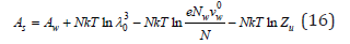
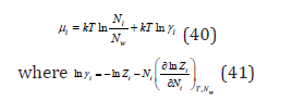
Differentiating Eq. (16) by the number of solvent molecules, its chemical potential in solution can be determined as
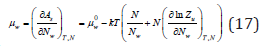
where  is the chemical potential of a pure solvent. Eq.
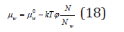
(17), considering Eq. (15), can be represented as
is the chemical potential of a pure solvent. Eq.
(17), considering Eq. (15), can be represented as
On the other hand, chemical potential of the solvent can be determined using the saturated vapor pressure above the solutions. Assuming that the solvent behaves like an ideal gas in gaseous phase, its chemical potential according to Eq. (1) and (7) can be expressed as
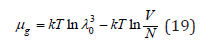
Next, using Eq. (9) we have
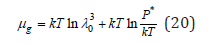
where P* is saturated vapor pressure above the solution. Similarly, for a pure solvent at a saturated vapor pressure Pw* we have
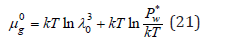
At phase equilibrium, the condition of equality of chemical potential is observed, i.e., μw = μ g for the solution, μ0w = μ0g for pure solvent. Then, using Eq. (20) and (21), the chemical potential of the solvent can be represented in the form Eq. (3)
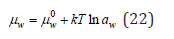
where 0w μ is the chemical potential of the pure solvent (the standard state), and aw is the activity of the solvent
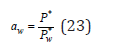
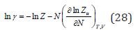
Comparing Eq. (18) and (22), osmotic coefficient can be determined as
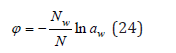
Eq. (24) obtained for dilute solutions extends to the entire domain of the existence of solutions and is the basis for the experimental determination of the osmotic coefficient. At the same time, it is necessary to make correction for the calculation of osmotic pressure. Comparing Eq. (14) and (15) in the region of an infinitely dilute solution, we have
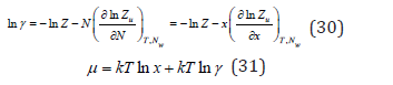
Differentiating Eq. (10) by the number of particles, it is possible to determine the chemical potential of the solute
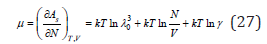
where γ is the activity coefficient
The first term of on the right side of Eq. (27) actually plays the role of some standard state, where under the sign of the logarithm is a quantity having the dimension of volume 3 [ ] λ0 v , and characterizing according to Eq. (21) the gaseous state of the solvent. Therefore, in solutions, considering the arbitrariness of the choice of the standard state, it is necessary to use another value 0w v is the molecular volume of the pure solvent. Then, the chemical potential of the solute can be expressed as
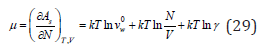
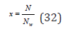
In dilute solutions, where it is possible to put v=Nw vw Eq. (28) and (29) respectively, take the form
where x is the relative concentration introduced by Debye [5]
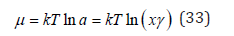
Using Eq. (32), the activity of the solute can be defined as a=xγ and represent Eq. (31) as
At constant pressure and temperature, the Gibbs-Dugem equation can be represented as [2]
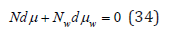
from where it is possible to establish a connection between the parameters of the solution [6]
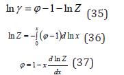
Eq. (35) – (37) remain unchanged for all types of solutions,
both molecular solutions and all types of electrolyte solutions
[3]. In binary solutions of electrolytes, where Np=qpN cations and Np=qpN anions are formed during dissociation, where 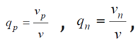 v = vp + vn are stoichiometric coefficients, so that the total number
of ions N = Np + Nn . In this case, Eq. (10) can be generalized and represented
as [3]
v = vp + vn are stoichiometric coefficients, so that the total number
of ions N = Np + Nn . In this case, Eq. (10) can be generalized and represented
as [3]
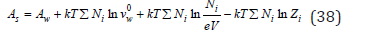
from where the chemical potential of each of the ions can be defined as
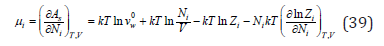
Turning to an infinitely dilute solution ( 0 ) V = Nwvw , Eq. (39) can be transformed to the form
Further, the average chemical potential in the relative concentration scale can be defined as
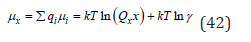
where 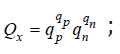 γ is the average ion activity coefficient
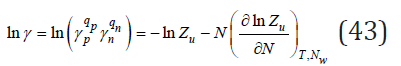
where 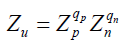 is partition function of the solution.
In electrolyte solutions, the concentration is usually defined as the number of moles of the starting substance related to 1kg of solvent, called molality m. The relationship of this value with the relative concentration is expressed
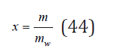
where mw is the number of moles of solvent contained in 1kg (for water mw=55.51mol/kg). Another concentration used is molarity, defined as the number of moles electrolyte in 1 liter of solution. The relationship of these concentrations is defined be the ratio
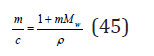
where Mw is the molecular weight of the solvent, ρ is the density of the solution. Using the Eq. (42) and (44), the chemical potential of the electrolyte in solution can be expressed as a function of molality
where  Mw is the standard state of solution, a is the
activity of the electrolyte
Mw is the standard state of solution, a is the
activity of the electrolyte 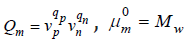
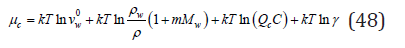
and further, using Eq. (45), as a function molarity
where Qc = Qm ; ρw is the density of the pure solvent.
Discussion
As follows from Eq. (29), he chemical potential of electrolyte is most strictly determined in the molar scale of concentration. However, this concentration significantly depends on temperature. Therefore, a result of which the overwhelming number of experimental data is expressed a molality concentration, which explains the procedure described above for converting data into molar concentration. When comparing the activity of different electrolytes in aqueous solutions, it is necessary to use uniform concentration scale, and the activity coefficient unchanged in any scale, and the activity of the component when using Eq. (46) and (48) has a concentration dimension. The latter circumstance is not an obstacle to this goal, since the standard state is function characterized by the parameters of a pure solvent, so that product of aiλ according to Eq. (2) - (4) is always dimensionless quantity. The structure Eq. (42) differ in that the properties of a pure solvent are included in the value of the electrolyte activity.
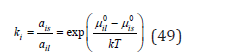
It follows from this that in all cases the state of a pure solvent is taken as a standard state. I this case, the main parameters of the electrolyte according to Eq. (35) – (37) take values Z→1; φ→1; γ→1. Note also that the chemical potential in an infinitely dilute solution remain indeterminate value, but this does not cause difficulties in calculating the energy of the system, since in this limiting case 0 lim ln 0 N N N → = and the free energy of the system corresponds to its value in a pure solvent. Turning to the evaluation of the interphase distribution function of components, let us consider a typical process of co-crystallization of impurity and main components in ternary water-salt systems. From the condition of equality of the chemical potentials of each component in the liquid μil and solid phases μil, the distribution coefficient can be determined according to Eq. (3) as
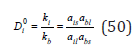
where μ0il , μ0is are chemical potentials in the standard state, ail , ais are the activity of the components in the liquid and solid phases, respectively. Composing the ratio of coefficients of the impurity ki and the main component kb, it is possible to determine the thermodynamics co-crystallization coefficient of the impurity component as
By choosing as a standard state in the solid phase for each component as the state of the pure component, Eq. (50) according to Eq. (49), can be converted to the form
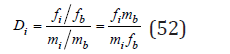
where a0il ,a0bl are the activity of the components in their binary saturated solutions. Turning to concentrations, we define the equilibrium coefficient of co-crystallization as the ratio
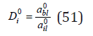
Where mi ,mb are the concentrations of the components in the liquid phase, fi ,fb are the molar fractions of the impurity and the main component, so that fi+fb=1 , moreover, for non-isomorphic compounds that do not form solid solutions, these values are the activities of the components in the solid phase : ais=fi; ais=fi. In the region of the micro-concentrations of the impurity component at mi → 0 also 0 abl → abl , from where comparing Eq. (50) and (51), we have
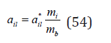
Here ail is the activity of the impurity component in the mixed solution, which under the same condition mi → 0 can be defined as [3,7]

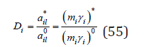
where * il a is activity of the impurity component in its binary isopiestic solution, at the same solvent vapor pressure as in the mixed solution, i.e., with the same solvent activity. Combining Eq. (52) – (54), we have
where the activities * ail , 0 ail are determined by Eq. (47). The results of calculations according to Eq. (55) are shown in Table 1. On the other hand, it is often found in the literature to determine the activity of the components of the liquid phase in the form [8]

where ν – stoichiometric coefficient of the electrolyte. In this equation, L is essentially the product of ionic activities, or the product of solubility for water-soluble salts. For example, for aqueous solution AgCl L 865 10 11 = × − , but solubility m L1 v 93 10 6 = = × − [9]. Indeed, the direct use of Eq. (56) for the examples in Table 1 leads to discrepancies with the measurement data be several orders of magnitude.
Conclusion
The conditions formulated above are necessary and sufficient for calculating and comparing the chemical potentials and activity of the components in solutions. In all cases the standard state of the chemical potential is related to parameters of the pure solvent and the activity of the components is proportional to their concentration in solution. This is the main difference between the proposed method and other methods based on some fixed or even hypothetical states of a system component. At the same time, the simplicity and clear physical meaning of the definition used make it possible to extend the proposed method for calculating of the chemical potentials in other equilibrium heterogeneous systems.
References
- Isihara A (1971) Statistical Physics. Academic Press, New York, USA.
- Landay L, Lifshitz E (1995) Statistical Physics. Nauka-Physmathlit, Moscow, Russia.
- Аllakhverdov G (2019) Thermodynamics of solutions and separation of elements during crystallization. Тriumph, Моscow, Russia.
- Prigogine I, Kondepudi D (1999) Modern Thermodynamics. John Wiley & Sons, USA.
- Debye P (1924) Osmotic equation of state and activity of diluted strong electrolytes. Phys Z 5: 97-107.
- Allakhverdov G (2008) Doklady Physics. 53(8): 420-424.
- Allakhverdov GR, Zhdanovich OA (2019) Thermodynamics of the ternary water-salt systems. Aspects in Mining & Mineral Science 4(3): 491-494.
- Robinson R, Stokes R (1959) Electrolyte Solutions. Butterworths, London, United Kingdom.
- Мironov V (1962) Radiochemical data on the solubility of silver chloride. Radiochemistry 4: 709-711.
© 2022 Grant Allakhverdov. This is an open access article distributed under the terms of the Creative Commons Attribution License , which permits unrestricted use, distribution, and build upon your work non-commercially.
Editor In Chief


.jpg)


Signup for Newsletter

Quick Links
 Editorial Board Registrations
 Submit your Article
 Refer a Friend
 Advertise With Us
Our Recent Edition

.jpg)


Top Editors


.jpg)


.bmp)
.jpg)
.png)
.jpg)


.jpg)


.png)

.png)


.png)


Financial Support

Sponsors

Latest e-Books

Latest Video

 a Creative Commons Attribution 4.0 International License. Based on a work at www.crimsonpublishers.com.
Best viewed in
a Creative Commons Attribution 4.0 International License. Based on a work at www.crimsonpublishers.com.
Best viewed in