The Appearance of Plasticity on the Blocks Surfaces in Porous and Cracked Media

The idea of creation of new model of space is the following. We consider some finite volume of body. In this case, the surface forces apply to sphere of radius l0 while the inertial forces apply into center of structure. There is no possibility to tend an elementary volume into zero and coincides points of surface and the point of inertial forces like in classical continuum. We must consider a finite volume like representative volume of body and we have a problem of different positions of surface and inertial forces. There is urgent necessary to translate surface forces into the center of structure by special translation operator. Obvious consequence of this action will be a possibility to apply the conservation law of ordinary mechanics into some image of structural continuum like in usual classical model of continuous media. Some results of new model of structured continuum published earlier [1], but it is necessary to repeated some formulas from [1] in order to present new idea about effect of equilibrium state for structured medium. This idea may be present more clearly by using previous results, because there is closed relation between them. It defines some model of a deformed continuous solid as the equation of equilibrium fulfills on the contour. It does not fulfill for the volume inside D as stress is absent from a part of the contour. Different gray shades correspond to compositionally different grains. The one-dimensional operator of field translation from point x into point x±l0 gives by symbolic formula [2]:

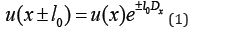
In this formula: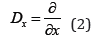

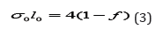
There is a relation between the average distance between one crack to another one (or one pore to another one) and the specific surface , namely

The analogous operator of translation for some sphere gives by expression:

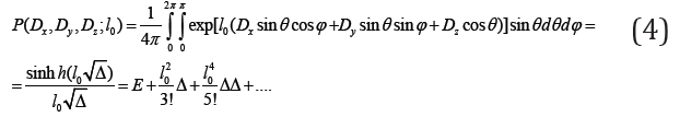
Here E is the unit operator. According to Poisson formula, we have [3]:

In addition, P operator rewrites as follows:

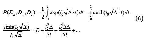
The P operator represents the operator of continuity. Classical Cauchy and Poisson continuous model of space means that P=E. In structured medium, the last relation is not valid. The equation of motion for blocked media with constant value published earlier [1] and gives by expression

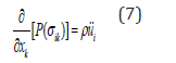
The more detailed form is following

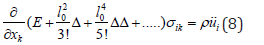
In one-dimensional situation and for case of stationary vibration this equation takes a form

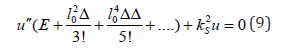
The substitution gives the dispersion equation for unknown wave number k, or for unknown wave velocity, which depends on range of structure l0 or specific surface of sample 0.

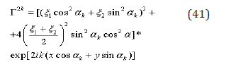
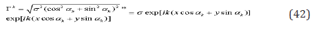
Instead of (7) in static, we have more simple equation, namely

The inverse operator from zero contains, besides of zero and constant value, some periodical functions, i.e.

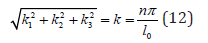
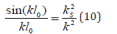
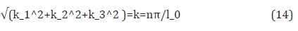
For dispersion equation (10) it means that 0 0 sin(kl ) = 0; k = nπ / l , where is the integer number.

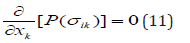
The equation of equilibrium (11), after acting of inverse operator 1 0 ( , , ; ) x y z P− D D D l , takes a form

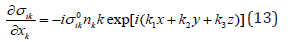
Here is the tensor of stresses, which corresponds to classic solution for a previous problem of elastic equilibrium, is a some random normal vector, and

The inhomogeneous equation (13) has a high oscillating right hand term, so it is equal to zero in average. This distinction from usual equation of equilibrium is relates with microstructures of real rocks. The right hand of (13) is the finite analog of the first derivative of Dirac delta function, which concentrated on the intervalfl_0 , where f is the porosity and l_0is the average distance from crack to its nearest neighbor. As to integer number n, it not bound formally, but it is value closed to l_0⁄δ , where δ- is an average crack opening or the second scale size (a thickness of plastic zone. The partial solution of equation (13) we can write in the form

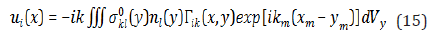
The symbol means the Green tensor of elastic equation of equilibrium, and there is a summation with respect to symbol Taking into account that linear size of structure sufficiently less, than a linear size of sample, we can reduce an integral (15) to Fourier transformation of the Green tensor [1], because we changed approximately finite area of integration into infinite one. This transform gives us the representation of partial solution in the form

Making a summation, we can write (16) in another form

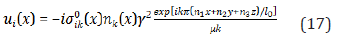
In the formulas (16,17) Cartesian coordinates of a point (x) in the exponent corresponds to stable point (x). There is a notation k / m m n = k k . The strains contain the first power of a wave number , not a second power. It causes the serious effects.

The tensor of stresses σ_ij (x) gives by expression

The stresses with different indexes contain the oscillating signs of normal, and the average value of them equal to zero. However, the normal stresses (an average square of cosine is equal to 1/3) can be represent in the form

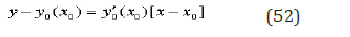
As to dilatation due to partial solution, it is represents by expression

The product of random normal components gives us in common case, the random amplitudes of stresses, while the squares of amplitudes in three-dimension space equal to one third, if the space is uniform. In this case, we have deterministic part of amplitude of dilatation and pressure

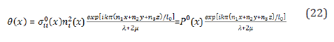
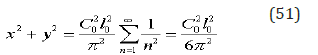
In the formula (22) is a pressure, which is corresponds to classic elastic solution. A series in (22) with respect to , is, in common case the divergent series, if the expression in the square bracket is an integer number. It corresponds to the strains localizing process. It means that there are some planes; where strains may not bounded grow. This condition is valid on the planes kind of

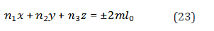
Here m is an integer number. Really, we may generalize the condition (23), for constructing the envelopes of planes and curves in two-dimensional case. The envelopes will be sliding surfaces or curves with not homogeneous stress-strain state. The simple condition (23) can generalize in the form

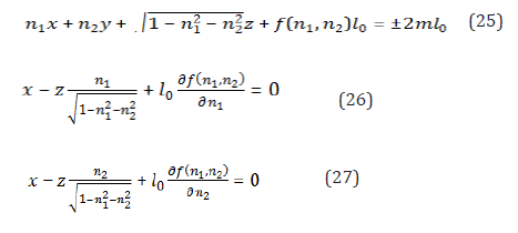
Heref(n_1,n_2 ) 〖 l〗_0 is the arbitrary function of mentioned variables. In this case, the main equation (1) is satisfied. The equations of envelope surfaces (lines in the two-dimensional case) take a form

Expressing in terms from equations (26) and (27), and substituting them in the equation (25) we get the envelope surfaces equations, and, in the two-dimension case, the envelopes curves ones of practically arbitrary complication. However, the alternation of odd and even terms in the exponent gives us the convergent series, because there is sign changing successful of summands, and there is no localization effects. It is valid when the condition (25) change to the condition

It means that we have different solutions, and the real of them must determine by additional requires.

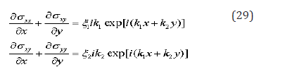
In this case, the equation of equilibrium takes a form

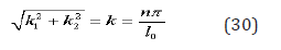
The space frequencies satisfy to equation, if is an integer number

As to arbitrary values we can put that they may be equal to the unit, or may be random values with the average values equal to zero. Let us try to find simplest solutions, which represent a constant field of stresses in average. Let us suppose that a solution me by represent in the form, where and are constants

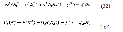
The substitution (31) into (29) gives the values of constants .

The system (7),(8) gives a field of displacement

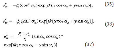
Here is . Strains represent by expressions

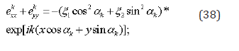
The plane dilatation looks like

If we put , the plane dilatation is

The second invariant of strain tensor takes an analogous form [3]

In this case, the first invariant of the strain tensor dilatation and the second one are the same. If we put that are random values with zero average quantity, we have the plane strain equal to zero, while the square of the second invariant of strain tensor takes a form

Taking into account that the average value of square of random value is equal to the variance of it, and the average value of product is equal to zero, we can represent the second strain tensor invariant by expression

The value is a variance of both random values . The summation of (42) with respect to the index gives us a Dirac delta function, which concentrates on the straight lines ,and these lines are orthogonal to each other. Shear strains are proportional to the variance of random strains. The solution (43) is analog of classical solution of a two dimensional plasticity [2] with incompressibility. However, we have the finite distance between mentioned straight lines, namely . Besides, of it, if we use the finite numbers of index , and the shear stress will equal to -the elasticity limit, we can determine the second size of microstructure, the finite thickness of sliding line. Formulas (36-42) give us partial solutions, which may be summate with any common solutions of two-dimensional elastic equilibrium equations. If we put the uniform distribution of random values the average deviation of them is , where is the intensity of the shear stresses, which get by solving of the usual elastic problem, and -is a porosity of blocked medium. We can put that the intensity of tangent stresses practically the same on the structure, while on the deforming body it depends on coordinates.

The plasticity is not valid, when the sum in the formula (43), not reach the elastic limit. However, it will be at a large value , and for lesser values ,we have more thick of sliding line, i.e. the second characteristic size of deforming structure. Thus in the case of transition from elasticity to incompressible plasticity in vicinity of sliding lines, the free terms are defined. The summation of strains with respect to index gives, at the limit, a Dirac delta-function on the some straight lines, where the argument in brackets is a constant value. Besides of it, there is a second condition, namely, the values are the same at the any index. It means that we put a scaling similarity. If there are , the summation of finite numbers of exponents gives some continuous function. This function has the sharp maximum (minimum) on the boundaries of squares or rhombs, which bounded the elementary grid with a period. It means that arrive two is ogonic straight lines assemblages, and there is elastic state between them. For , these assemblages are orthogonal, i.e.

Figure 1: Meso-structure contoured by С centered on O.

The elastic behavior of a main mass of medium corresponds to common solution of the usual elastic problem. In vicinity of boundaries of grids, which is making of slide lines is acting the special solution, which represents by formulas (31-40). Hence, the solution of problem for structured medium gives us the grid structure of stresses, where in the main part of volume there is a usual elastic state, while in vicinity of sliding lines there is a plastic flow state. We can put the shear stresses on the sliding lines equal to limit of shear elasticity .Here is the elastic limit of tangent stress, and is an analogous limit for shear strain. The Figure1 shows the configurations of sliding lines for uniform stress-strain situation in average. The every figure corresponds to some number .The more a number ,the thinner sliding lines. This situation is analog of rigid plasticity with uncompressed material. The vanishing of pressure in vicinity of sliding lines is decreasing the friction in mentioned lines. There is a question about value of k, which is sufficient for mentioned state. The displacement field in elastic distinguishes from such field in plastic zone. This distinction determines by the value . The break of strain determines by expression . Here is a thickness of sliding line (the second scale level). The strain into plastic zone is . It means that there is . It gives a possibility to determine the integer number . Hence, we have a state similar to plastic state in the simplest constant stresses in average. The role of rectangular grids is similar to the role of characteristics of plastic flow or sliding lines by simple stress state. However in classic plasticity the characteristics occupied the all space, and in structured continuum there is a finite distance between lines of grids, with the period, equal to

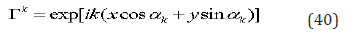
The common structure of displacement field in two-dimensional space we can represent as a product of arbitrary amplitude to the exponential phase function

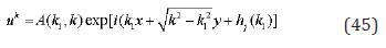
This phase function may be very large, if the volume of body much more than a volume of structure. Besides, of it, this function is constant at the condition

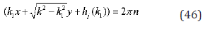
Here n is an integer number. The envelope curve arrives by additional condition

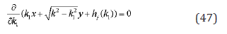
and the joint resolution of (46) and (47) gives the envelope of straight lines (44).

The parametric equation of envelopes curves takes a form

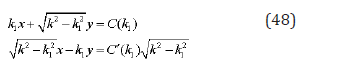
Eliminating the parameter from two equations (48), we can get the explicit form of assemblage curve like The isogonic assemblage of straight lines of different orientation correspond isogonicassemblage of envelopes. For example, if in (48) is a constant value, the elimination of the parameter gives us a circle

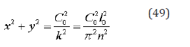
I.e. there is the envelope of centered stress field, which is analogous field in classic plasticity.

The expression (45) in the case (48) looks like

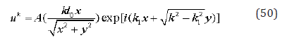
In the formula (50), the amplitude depends on the polar angle, and we get a representation the centered field of stresses and strains like in classic plasticity [4]. A summation with respect to in (50) gives us a formula

Assuming we get a circle with a radius equal to .

The more complicate example gives us the assemblage of straight lines, with assemblage of ellipses as envelopes. Really, an equation of straight line, which is the tangent to the ellipse, is

The equation (53) after simple transformations takes a form

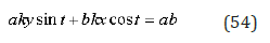
Hence, the envelope curve equation looks like

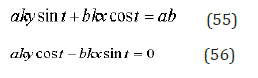
The elimination of a variable from equations (55) and (56) gives the envelope equation kind of

The orthogonal trajectories are assemblages of hyperbolas. The parameters and are discrete ones. It means that the envelopes divided to each other by finite distance, and they not occupy all space, only the infinite small part of it Figure 2. The appearance of inhomogeneous periodical stresses and strains due to structures in homogeneous mrdium in average. The integer number n is equal to 10 Figure 3. The appearance of two characteristic scales in structured body, the distance between slide lines and -the thickness of plastic zone, the integer n is equal to 25. Figures 4a-4f illustrates the successive increasing of elastic area (white color) of a body with simplest common stress, and the concentration of plastic zones near sliding lines. The integer n is equal from 30 up to 100.

Figure 2: The appearance of inhomogeneous periodical stresses and strains due to structures in homogeneous mrdium in average. The integer number n is equal to 10.

Figure 3: The appearance of two characteristic scales in structured body, the distance between slide lines and -the thickness of plastic zone, the integer n is equal to 25.

Figure 4: Illustrate the successive increasing of elastic area (white color) of a body with simplest common stress and the concentration of plastic zones near sliding lines. The integer n is equal from 30 up to 100.

The infinite order of equilibrium differential equations gives us a possibility to describe the model of deforming, where the main volume of a structured body practically have no any strains, and all strains concentrate near thin layers in vicinity of structure contacts.

The localization of stresses and strains in structured media begins in elastic state of deforming.

The small areas of a stress-strain concentration looks like usual orthogonal sliding lines in classic plasticity. However, they have a finite effective thickness, which depends on the average size of structure and the limit elastic strain. Besides, of it, there is a finite distance between analogs of sliding lines, which is equal to the average distance from one pore to another one, or between cracks.

The energy of transition from elasticity to plasticity may be very small, because the main part of a body volume is in elastic state. The plasticity area occupies very small part of mentioned volume.

1. Sibiryakov BP, Prilous BI, Kopeykin AV (2013) The nature of instability of blocked media and distribution law of unstable states. Physical Mesomechanics 16(2): 141-151.
2. Maslov VP (1973) Operator methods. Operational Method.
3. Gradstein IS, Ryshik IM (1963) Tables of integrals, sums, series and products.
4. Sibiryakov BP (2015) The appearance of plasticity on the blocks surfaces in geological media. AIP Conference Proceedings 1623: 579.