
- About Us
- Information
-

The Author ensures that the research has been conducted responsibly and ethically with adherence to all relevant regulations. read more..
- For Authors
- For Reviewer
- Manuscript Guidelines
- Membership
- Publication Ethics
-
- Journals
- Reprints
- e-Books
- Videos
- Policies
- Contact Us
 COVID-19
- Submissions


Full Text
Aspects in Mining & Mineral Science
A Granular Flow Model for Tumbling Mills: Dry Mill Power
Tupper GB1,2*, Govender I3, Richter MC4 and Mainza AN4
1Department of Physics, University of Cape Town, South Africa
2Associate Member, National Institute for Theoretical Physics, South Africa
3Department of Chemical Engineering, University of KwaZulu-Natal, South Africa
4Department of Chemical Engineering, University of Cape Town, South Africa
*Corresponding author: Tupper GB, Department of Physics, University of Cape Town, South Africa,
Submission: March 19, 2018;Published: March 29, 2018

ISSN 2578-0255Volume1 Issue4
Abstract
We develop a simple granular flow model for the dissipative power density and power draw in dry tumbling mills. The model is based on a Herschel-Buckley like granular rheology with a yield stress proportional to the pressure. Data obtained from Positron-Emission-Particle-Tracking is used to correlate dependence on fill, speed and lifters.
Keywords: Power; Efficiency; Granular; Rheology; PEPT
Introduction
Tumbling mills play a crucial role in many industries. Such mills account for some 60% of operating costs, but are only <5% efficient in comminution [1]. Hence even incremental increases in efficiency hold the promise of enormous savings. To achieve improved efficiency it is natural to seek a better understanding of the processes taking place inside the mill. Unfortunately, the aggressive opaque environment of a milling operation does not afford direct access to the mechanical environment. Consequently, most models are formulated from empirical measurements. Such empirical models can be tuned to provide highly robust descriptions; however, their specialised nature negates the ability to extrapolate beyond the mode of operation for which they were determined.
In recent year’s novel techniques like Positron-Emission-Particle-Tracking (PEPT) [2], and X-ray imaging, [3], have allowed researchers an in-situ perspective of particle dynamics deep within the charge body. Both systems are specialised to provide 3D trajectory fields, however, unlike the X-ray imaging system PEPT allows the use of real charge within a scaled industrial mill. PEPT uses particles labelled with β+ emitters (the tracer), the subsequent annihilation of the positron with an electron produces 511 keV back-to-back gamma pairs. Detection of a few such pairs provides the raw data for tracking the in-situ flow field of the tracer through opaque environments. Through PEPT one can build up time-averaged velocity andsolids concentration fields, as illustrated in Figure 1. In particular, the free surface of the charge is quantitatively discernable as a sharp transition in the solids concentration. With PEPT one can also find the shear rate distributions, but cannot directly access the shear stress. Recently PEPT has been used in the development of a power draw model based on the lever arm approach, Bbosa et al. [4].
Figure 1: Example of processed PEPT data for velocity field normalised to the mill shell velocity; arrows give direction and colours give magnitude. Black line represents the free-surfaces.

In this paper we use PEPT data in conjunction with a new granular flow model for the charge in the tumbling mill. The use of a continuum description of granular material is hardly new; it underlies the Eulerian-Eulerian approach to multi-phase flows in Computational Fluid Mechanics (CFD). Rajchenbach [5] used the Bagnold [6] rheology to study avalanches of mill charge. Taberlet et al. [7] assumed a Newtonian-like rheology supplemented with end wall friction to describe the free surface shape. Common to both is the assumption of rigid body motion below the equilibrium surface in contradiction to the definition of the equilibrium surface as the velocity does not vanish there.
What is novel here is, first, that we use a simple granular rheology inspired by recent developments in granular flow theory which amounts to a Herschel-Buckley model but with a yield proportional to the pressure. Second, by cutting the charge into thin slices in which the flow is treated analogously to an incline we obtain simple formula for shear rate and shear stress–hence also forth edissipative power density–that apply out to the mill shell. The importance of the dissipative power density in comminution is that, unlike the power draw, it gives a measure of the distribution of power available for liberation. Moreover, unlike Eulerian CFD, everything can be implemented on an ordinary laptop.
The balance of this paper is organised as follows: in Section 2 we develop our granular rheology[1]. In Section 3 we apply this rheology to the mill. Section 4 describes the PEPT experiments, which we analyse using our model in Section 5. Section 6 gives our conclusions.
[1]For a review of granular rheology in mills see Govender [12].
Granular Rheology
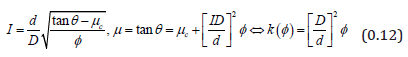
The theoretical study of granular flows can be traced back more than 60 years to the seminal work of Bagnold[1] [6,8]. Just over a decade ago the appearance of the seminal papers of Midi & da Cruz et al. [9,10], and the “granular rheology” due to Jop et al. [11], revitalised the subject[2]. The essence of the new rheology is that the dimensionless ratio of the shear stress to pressure as well as the solids concentration are in turn functions of the so-called inertial number:
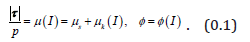
In that vernacularis termed the “friction coefficient”. The inertial number is the ratio of the time scale of rearrangement for spheres of diameterand mass density , and the shearing time scale :
More recently the Jop-type rheology has been shown to be constrained by the criteria of being well-posed, Barker et al. [15].
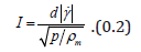
Now, the Jop et al. [11] split into static and kinetic frictions has a fluid analogy: is related to a Drucker–Prager yield criterion. Since dimensional arguments play a key role in Midi [9] it useful to see how the Bagnold [6] rheology thereby arises. If one makes the obvious assumption that a granular flow is non-Newtonian then
The ratiowhere  has dimension
  and since
  () is the only intrinsic length (inverse time)
 ; the dimensionless proportionality constant can only be a function of whence
  . According to Bagnold, 1956
  where
where 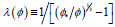 is the “linear grain concentration” and (close to for random close packing)[3].
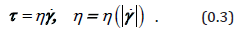
Of course that isn’t the whole story because it does not include the existence of the yield stress. To fix that one most simply imitates theHerschel-Buckley generalization of the Bingham model:
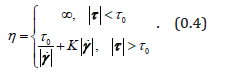
For the familiar cases of Bingham fluids, the yield stress is an independent constant determined by the cohesive interactions of the constituents. Clearly that is not the case for e.g. dry smooth spherical beads, and one reasons thatshould vanish in the absence of compression in that case. The simplest way to model that is to take the yield stress proportional to the pressure: . One thus arrives at
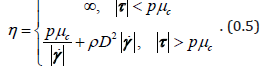
Here we have introduced a rheological diameter by  such that
  is the superficial mass density. In the context of the Bagnold [8] bed load theory the yield term can be viewed as a shear thinning fluid
[1]For a retrospective see Hunt et al. [13].
[2]For a review see Forterre & Pouliquen [14].
[3]We note that an alternative to Pouliquen et al. [16] is where the difference of random close and simple cubic is packing.
Mill Model
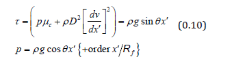
Consider now the application of our rheology to the tumbling mill. We construct at a point a local coordinate system with tangent to the free surface 5, subtending angle θ with ˆx , and ˆx′ pointing into the bed, as illustrated in Figure 2.
The lab coordinates are related to the local ones as
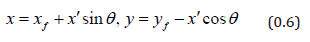
On the free surface
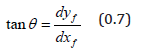
Hence, as f y is a function of f x , the independent variables are , f x x′ . Nowwe will make the small curvature or lubrication approximation: with x′ = h the depth that the mill shells, f s the displacement along the fee surface, and f R the radius of curvature of the free surface
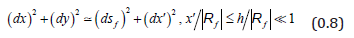
Assuming that the flow is stationary, parallel to the free surface and independent of f s or z 6, the equations describing the flow are
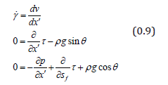
Assuming φ also constant , integrating into the bed with freesurface boundary conditions and the rheology (0.5) gives
Hence the shear rate is
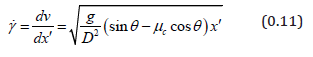
We note that the friction and inertial number are depth independent:
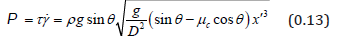
Since our local coordinates are a translation and rotation, the dissipative power density is
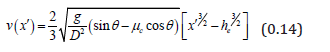
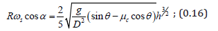
Integrating (0.11) subject ( ) 0 e v h = to at the equilibrium surface
Continuing this description out to the mill shell, we have that the flux per unit mill length vanishes:
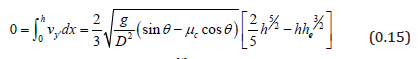
Then we have ( )2 3 2 5 0.543 e h = h = h . In general, the x′ axis is not aligned with the normal to the mill shell; see Figure 2. Further, even if it is there may be slip–see Figure 1a. Denote s ω =ωΩ as the angular ‘slip speed’. Hence the velocity x′ = h at is related to the mill radius R and mill angular speed ω by
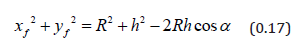
The angle α is related to ,ff x y as
Finally, the dissipative power density can be usefully reexpressed as
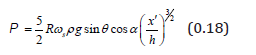
Figure 2: The proposed granular flow model structure.

Note that this is independent of particle size. Because of the non-Newtonian rheology this grows faster than the shear rate that is often used as guide to liberation in comminution. To obtain the total power per unit length one needs to observe the global measures are different owing to the boundaries
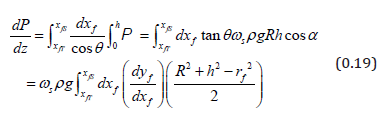
Integrating by parts
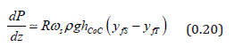
Herein CoC h is the depth measured along a radial line through the Centre of Circulation, and tan CoC θ is the free surface slope there, while fS y ( fT y ) is the mill shell y − coordinate at the shoulder (toe).When the mill is static the charge forms a segment subtending T S α +α ; the stationary flow displaces the shoulder and toe such that sin ( ) fS CoC S y R θ −α and sin ( ) fT CoC T y −R θ +α where / cos 2 S T CoC α h R . Hence
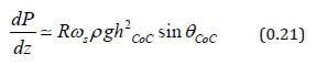
Since what goes in must come out, (0.21) is also a formula for power draw per unit length.
Figure 3: Left, experimental mill employed in positron emission particle tracking experiments. Centre, mill lifters geometry. Right, the right image illustrates the PEPT Siemens EXACT 3D scanner.

We will consider PEPT data with lifters was acquired by scanning a model mill of R=0.150 m and length of L=0.3 m with lifters varying in height (1.5, 3, 6 and 10 mm), containing 20%, 30% and 40% volumetric filling of 5 mm borosilicate glass ballotini and introducing a drilled and activated representative glass bead tracer to track with the Siemens EXACT3D scanner. The mill was run at 55, 70 and 85 % of critical speed. The tracer was activated with a resin bead that was subjected to an ion-exchange reaction using 68Ga isotope with an activity of no more than 1mCu, allowing for a tracking time of up to 2 hours.
The charge velocity field can be directly obtained by differentiating the trajectory data. The determination of the solids concentration distribution is based on the methodology of Wildman et al. [16]: the mill volume is partitioned into rectangular voxels; the number density in a voxel j of the mill is given by
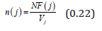
Here N is the number of particles, F ( j) is the residence time fraction of the tracer in voxel j , and j V is the volume of the voxel. With j t is the time spent by the particle in a given voxel andT the total system observation time, the residence time fraction - or the fraction of total observation time a particle spends in a particular segment - is given by:
The solids concentration φ in voxel j is then given by:
Model PEPT Data Analysis
To begin, it is useful to take the mill angular speed ω in units of the critical speed c ω = g R for centrifuging, and lengths in units of the mill radius R . These natural units amount to setting R = g =1 in the formula (Figure 4).
Figure 4: Dimensionless dissipative power density with 3mm lifters at three volumetric fillings.

We start with the dissipative power density (0.18) since this is independent of rheological size. Indeed, the dimensionless
with taken from PEPT can only depend on volumetric fill. The results are displayed in Figure 4. One notes similarities to the power draw density maps of Bbosa et al. [4]–the primary difference is that the power draw maps show an enhancement around the CoC that is absent in the dissipation mapsSince it involves lifters and the speed typical in comminution it is most telling that this is strongly peaked in a short narrow band near the mill shell. One thus begins to understand why the comminution tumbling mill has a low efficiency in liberation.
In application, one needs to know not only the mill radius and charge density, but also the dependence of slip on fill and lifters. We have measured the slip just above the lifters along the radial line through the centre of circulation (Coc). Further , one needs correlatios of CoC h and cos CoC θ . The results are summarised in Figure 5, along with the predicted dimensionless dissipative power per unit length (Figure 5).
Figure 5: Measured(a) slip Ω , (b) bed depth CoC h (c) free surface slopetan CoC θ and (d) dimensionlrss power per unit length for different fills and lifter sizes.

Figure 6: Dimensionless dissipative power density ( ) s P Rω ρ g for 20% fill with 1.5mm, 3mm, 6mm, and 10mm lifters (left to right) at 55%, 70% and 85% critical speed (top to bottom).

The trend in Figure 5 is clear: reducing the fill significantly reduces the total dissipative power and, since what goes in must come out, also the power draw. At 20% fill, the 1.5mm lifters for 5mm beads are obvious outliers; to confirm this we display the full suite of maps in Figure 6–one notes the higher liberation zone is squeezed into a vanishingly thin strip. In the other cases, higher lifters and/or speed enhance the higher liberation zone.
Conclusions
In this paper we have developed a granular flow model for the tumbling mill, based upon a n = 2 Herschel-Buckley type rheology with a yield stress proportional to the pressure. Using a local coordinate system tangential to the free surface we formulated and solved the non-Newtonian Navier-Stokes equations to obtain shear rate and shear stress–hence also the dissipative power density. We further obtained an expression for the total dissipative powerwhich is to say power draw-per unit length. We have not validated the total power here due to absence of corroborating measurements for the extensive data set considered.
While a number of simplifying assumptions and approximations were involved, the model’s basic equations can be quickly solved by anyone on any laptop (and some tablets) provided a model for the free surface such as Taberlet [7] is assumed. Finally it must be reminded that the model is restricted to dry systems in the sense that the Bagnold [6] number is large; the extention to wet systems involves a number of issues beyond those addressed here. Similarly,understanding the free surface necessitates a more refined treatment of the structures exposed in Figure 1, similar to Bagnold’s [8] bed load theory.
Acknowledgement
This work was supported by Anglo American. The work of G. B. Tupper was partially supported by a grant from the National Research Foundation.
References
- Wills A (1997) Mineral Processing Technology: An Introduction to the Practical Aspects of Ore Treatment and Mineral Recovery. Oxford
- Parker DJ, Dijkstra AE, Martin TW, Seville JPK (1997) Positron emission particle tracking studies of spherical particle motion in rotating drums. Chem Eng Sci 52 (13): 2011-2022.
- Govender I, McBride AT, Powell MS (2004) Improved experimental tracking techniques for validating discrete element method simulations of tumbling mills. Journal of Experimental Mechanics 44(6): 593-607.
- Bbosa LS, Govender I, Mainza AN (2016) Development of a novel methodology to determine mill power draw. International Journal of Mineral Processing 149: 94-103.
- Rajchenbach J (1990) Flow in powders: From Discrete Avalanches to Continuous Regime. Phys Rev Lett 65(18): 2221-2225.
- Bagnold RA (1954) Experiments on Gravity-Free Dispersion of Large Solid Spheres in a Newtonian Fluid under Shear Proceedings of the Royal Society A 225(1160): 49-63.
- Taberlet N, Richard P, Hinch EJ (2006) S shape of a granular pile in a rotating drum. Physical Review E 73: 050301(R).
- Bagnold RA (1956) The flow of cohesion less grains in fluids. Philosophical Transactions of the Royal Society of London A 249(964): 235-297.
- GDR Midi (2004) On dense granular flows. Eur Phys J E14(4): 341-365.
- da Cruz F, Emam M, Prochnow M, Roux JN, Chevoir F (2005) Rheo-physics of dense granular materials. Phys Rev E72: 021309.
- Jop P, Forterre Y, Pouliquen O (2006) A constitutive law for dense granular flows. Nature 441(8): 727-730.
- Govender I (2016) Granular flows in rotating drums: A rheological perspective. Min Eng 92: 168-175.
- Hunt ML, Zenit R, Campbell CS, Brennen CE (2002) Revisiting the 1954 suspension experiments of R. A. Bagnold.Journal of Fluid Mechanics 452: 1-24.
- Forterre Y, Pouliquen O (2008) Flows of Dense Granular Media. Annu Rev Fluid Mech 40: 1-24.
- Barker T, Schaeffer DG, Bohorquez P, Gray JMNT (2015) Well-posed and ill-posed behavior of the µ(I)-rheology for granular flow. J Fluid Mech 779: 794-818.
- Wildman RD, Huntley JM, Hansen JP, Parker DJ, Allen DA (2000) Single-particle motion in three-dimensional vibro fluidized granular beds. Phys Rev E Stat Phys Plasmas Fluids Relat Interdiscip Topics 62(3): 3826-3835.
© 2018 Tupper GB. This is an open access article distributed under the terms of the Creative Commons Attribution License , which permits unrestricted use, distribution, and build upon your work non-commercially.
Editor In Chief


.jpg)


Signup for Newsletter

Quick Links
 Editorial Board Registrations
 Submit your Article
 Refer a Friend
 Advertise With Us
Our Recent Edition

.jpg)


Top Editors


.jpg)


.bmp)
.jpg)
.png)
.jpg)


.jpg)


.png)

.png)


.png)


Financial Support

Sponsors

Latest e-Books

Latest Video

 a Creative Commons Attribution 4.0 International License. Based on a work at www.crimsonpublishers.com.
Best viewed in
a Creative Commons Attribution 4.0 International License. Based on a work at www.crimsonpublishers.com.
Best viewed in