Production Scheduling in Block Caving with Consideration of Material Flow

Any planning and financial analysis in a mining project depend on production schedule in which the amount of ore and waste removal is determined in each period. An optimum realistic production schedule can significantly improve the overall practicality and profitability of the project. Block-cave mining operation is involved with uncertainties which cannot be ignored in the production scheduling; while the caving is occurring, the flow of material (which happens because of the gravity) can be unpredictable. The flow of material will result in grade and tonnage uncertainties in the production during the life of mine. Numerical methods are useful tools to model the material flow. Stochastic optimization can capture the uncertainty of material flow while optimizing the production schedule.

Production schedule in a block-cave mining operation can be investigated from different levels of resolutions: cluster level, draw point level, or slice level [1]. In this research, the slices are the smallest production units. The output of the production schedule at this level would be the periods in which each of the slices within a draw column is extracted and sent to the processing plant. These decisions are made based on the defined goal(s) in the objective function while considering the limitations of the operations as the constraints of the model. The proposed production scheduling model is a stochastic optimization model in which the net present value of the project is maximized during the life of the mine while the deviations from a target production grade are minimized. Different scenarios of the grade for the slice model are generated to capture the uncertainty of the production-grade which exists because of the material flow during production.

Currently, most of the surface mines work in a higher stripping ratios than in the past. In some conditions, a surface mine can be less attractive to operate, and underground mining is used instead. These conditions are (i) too much waste has to be removed in order to access the ore (high stripping ratios), (ii) waste storage space is limited, (iii) pit walls fail, or (iv) environmental considerations could be more important than exploitation profits [2]. Among underground methods, block-cave mining, because of its high production rate and low operating costs, could be considered as an appropriate alternative. Projections show that 25 percent of global copper production will come from underground mines by 2020. Mining companies are looking for an underground method with a high rate of production, similar to that of open-pit mining. Therefore, there is an increased interest in using block-cave mining to access deep and low-grade ore bodies. A schematic view of block cave mining is shown in Figure 1.

There is a significant amount of research on production scheduling in mining operations, mostly in open-pit mining [2]. In block-cave mining, the production schedule determines which draw points to be opened/closed in each period, which slices to be extracted, what the best direction for mining development is, and what is the production rate and the production-grade during the life of mine. A detailed literature review of production scheduling in block-cave mining can be found in Khodayari & Pourrahimian [3].

Figure 1: Block cave mining [3].

Compare to open pit mining, production schedule in block-cave mining is more complicated to be optimized, mainly because of the material flow and its uncertainties. Researchers have been trying to model the flow of material and how it can impact the production in cave mining for almost three decades. Numerical models [1,4,5]; pilot tests [6,7] and full scale experiments [8-10] have been used to study the flow of the material. Pilot models have many limitations and in most cases cannot describe the behavior of the flow. Full-scale methods are usually expensive to use. Numerical models can be more efficient and less expensive if they are properly modeled [11]. Used Pascal cone to understand the probabilities of blocks moving down as the production occurs in caving operations. Although this model was dependent on the cell size and the probabilities, it was shown that stochastic models could be used to present the behavior of material flow.

This research proposes a stochastic optimization model in which, the uncertainty of the material flow which results in production-grade uncertainty, is implemented in the production scheduling optimization. This optimum production schedule will not only maximize the NPV of the project but also minimize the deviation of the production-grade from a target grade in all scenarios.

The proposed model maximizes the NPV of the mining project during the life of mine while trying to minimize the deviations of production grade from a defined target grade. To be able to capture the uncertainty of production in block-cave mining, the model is a stochastic optimization in which different scenarios of grade mixing are considered. The formulation of the objective function was inspired by a stochastic optimization model which was used by MacNeil & Dimitrakopoulos [12] for determining the optimal depth of transition from open pit to underground mining. The scenarios are defined based on the grade distribution in the mine reserve. Each scenario represents one circumstance that can happen during the production based on the flow of the material. Figure 2 shows the flow of the material and how it can impact the production.

Figure 2: Flow of the material and its impact on the production grade.

While extracting from a draw point, the material can move not only from the column above (DC8) but also from the columns in its neighborhood (DC1... DC7) into the intended draw point. The unpredicted material movements during the caving are the main source of the uncertainties in the operations. A production schedule would be more realistic if the uncertainties are captured. As it was mentioned, the decision units for the production schedule are the slices; the slice model is built based on the resource block model, the column above each draw point is divided into slices. In this section, the mathematical programming model is presented in details.

Notation

Indices:

t∈{1,....T} Index for scheduling periods

sl∈{1,...,Sl} Index for individual slices

dp∈{1,...,Dp} Index for individual draw points

s∈{1,.....S}Index for individual scenarios

a∈{1,...,A} Index for the adjacent draw points

Variables:

X^t_sl∈ Binary decision variable that determines if slices l is extracted in period t[ X^t_sl = 1 ]or not X^t_sl = 0

Y^t_dp∈{0,...,1} Binary decision variable which determines whether draw point dp in period t is active [Y^t_dp =1] or not [y^t_dp = 0]

Z^t_dp∈{0,...,1} Binary decision variable which determines whether dpat period t (periods 1, 2,..,t) has started its extraction [Z^t_dp=1] or not [Z^t_dp=0]

d^t_ls∈{0,...,∞} Deficient amount from the target grade (the metal content)

Model parameters:

^g_sl Copper (Cu) grade of slice sl

^gE Expected copper grade based on all scenarios

^tonsl Ore tonnage of slice sl

t_c Current period

sl_dp Number of slices associated with draw point dp

Input parameters:

TarGrade The target grade of production which is defined based on the production goals and processing plant s requirements

M_min Minimum mining capacity based on the capacity of the plant and mining equipment

M_max Maximum mining capacity based on the capacity of the plant and mining equipment

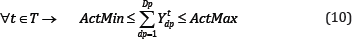
ActMin Minimum number of active draw points in each period

ActMax Maximum number of active draw points in each period

M An arbitrary big number

MinDrawLife Minimum draw point life

MaxDrawLife Maximum draw point life

DR_Min Minimum draw rate

DR_Max Maximum draw rate

IntRate Discount rate

RampUp Ramp up

ScenNum Number of scenarios

^DPd^tp^c Draw point depletion percentage which is the portion of draw column dp which has been extractedfromdrawpointdp till period tc

Price Copper price ($/ tonne)

Cost Operating costs ($/tonne)

^C_u Cost (penalty) for excessive amount ($)

C_l Cost (penalty) for deficient amount ($)

Objective function

The objective function is defined as follows:

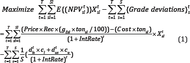
The first part of the objective function maximizes the NPV of the project during the life of mine by finding the optimum sequence of extraction for the slices in the mine reserve. The second part minimizes deviations of the production-grade from the target grade in different scenarios during the life of mine; thisis done by allocating penalties to the deviations that might happen in different scenarios.

Constraints

Operational and technical constraints of block-cave mining operations are considered to control the outputs ofthe optimizations model.Some decision variables depend on the number of draw points and the number of slices in each draw point.

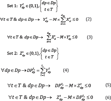
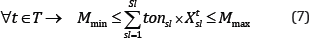
Logical constraints: There are two sets of binary decision variables in the proposed model which will be required for defining different constraints. Logical constraints connect the continuous decision variables to the binary ones, each set contains two inequality equations.

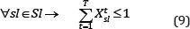
Mining Capacity: Mining capacity is limited based on the production goals and the availability of equipment.

Production-grade: This constraint ensures that the production grade is as close as possible to the target grade in different scenarios. The deviations from the target grade for all scenarios in different periods of production during the life of mine are considered for this constraint.

Reserve: This constraint makes sure that not more than the mining resources can be extracted, the output of the model would be the mining reserve.

Active draw points: A limited number of draw points can be in operation at each period; the mining layout, equipment availability, and geotechnical parameters can define this constraint.

Mining precedence (horizontal): The precedence is defined based on the mining direction in the layout. Production from each draw point can be started if the draw points in its neighbourhood which are located ahead (based on the mining direction) has already started their production. Equation (11) presents this constraint.

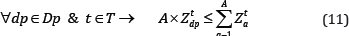
Where A is the number of draw points in the neighbourhood of draw point dp which are located ahead (based on the defined advancement direction), and Z is the second set of binary variables.

Mining precedence (vertical): This constraint defines the sequence of extraction between the slices within the draw columns during the life of mine.

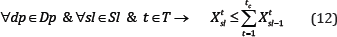
This equation ensures that in each period of t, slicesl(in the draw column associated with draw point dp)is extracted if slice sl-1 beneath it is already extracted in the periods before or during the same period(t_ic).

Continuous mining: This constraint guarantees continuous production for each of the draw points during the life of mine. In other words, if a draw point is opened, it is active in consecutive years (with at least the minimum draw rate of DRMin)till it is closed.

Draw rate: The total production of each draw point in each period of t is limited to a minimum and maximum amount of draw rate.

Draw life: Draw points can be in production during a certain time which is called draw life. The draw life is limited to the minimum and maximum years of operations by the following equation:

Solving the optimization problem

The proposed stochastic model has been developed in MATLAB [13] and solved in the IBM ILOG CPLEX environment [14]. CPLEX uses branch-and-cut search for solving the problem to achieve a solution within the defined mip gap (or the closest lower gap). The case study in this research was solved by a gap of 3% (a feasible integer solution proved to be within three percent of the optimal).

Figure 3: Draw points layout (circles represent draw points).

The proposed model was tested on a block-cave mining operation with 102 draw points. It was a copper-gold deposit with the total ore of 22.5 million tones and the weighted average grade of 0.85% copper. The draw column heights vary from 320 to 351 meters. Figure 3 & Figure 4 show the draw points layout (2D) and a conceptual view of the draw columns (3D).Each draw column consists of slices with the height of 10 meters (33 to 36 slices for each draw column). In total, the model was built on 3,470 slices. The goal is to produce a maximum of 2 million tones of ore per year during the ten years of mine life. The details of the input parameters for the case study are presented in Table 1.

Figure 4: A conceptual view of the draw columns.

Table 1: Scheduling parameters for the case study.

In this case study, different scenarios were defined by generating random numbers in MATLAB; a linear function was defined based on the original grades of the slices to produce different scenarios. The model was built in MATLAB (R2017a) and solved using IBM/CPLEX (Version 12.7.1.0). Also, the model was solved as a deterministic model in which there was no penalty for deviation from defined target grade. The production-grade in different scenarios (stochastic model) and deterministicmodel is shown in Figure 5

Figure 5: Average production grade based on the stochastic and deterministic models.

It can be observed that in all scenarios the production grade is as close as possible to the defined target grade during the life of mine. The deterministic model tries to maximize the NPV and the higher-grade ore is extracted at the first years of production and then the lower grades at the latter years. The mining capacity constraint regulates ore production, and the ramp-up and ramp- down are almost achieved in both stochastic and deterministic models (Figure 6 & Figure 7).

Figure 6: Ore production during the life of mine (stochastic model).

Figure 7: Ore production during the life of mine (deterministic model).

Horizontal precedence, which is the sequence of extraction between draw points, was achieved for both of models based on the defined V-shaped precedence (Figure 8 & Figure 9).

Figure 8: Ore production during the life of mine (deterministic model).

Figure 9: Sequence of extraction for draw points based on the deterministic model (2D precedence).

Figure 10: Sequence of extraction for slices in draw column associated with draw point 75 (numbers represent ID of slices within the draw column).

Vertical precedence determines the sequence of extraction between slices in each of draw columns. Figure 10 shows the sequence of extraction in draw column number 75. Extraction from this draw point starts from year 5 and ends at year 8; the sequence of extraction is from bottom to top, and the production is continuous which means that both the vertical precedence and continuous mining constraints were satisfied. The original height of draw column number 75 is 330.1 meters with the total ore of 212,397 tonnes which contains 34 slices. Based on the optimization results (Figure 10), the optimum height of draw or BHD (Best Height of Draw) was 260 meters with the optimum draw tonnage of 168,650; this means that 26 out of 34 slices are extracted during the life of mine.

Number of active draw points and number of new draw points which are opened in each year for both models are presented in Figure 11 & Figure 12. Comparing the new draw points to be opened in each year for two models, the stochastic model does not suggest big changes from one year to another while the deterministic model shows such a pattern. In other words, the results of the stochastic model are more practical than the deterministic model. A brief comparison among the original ore resource model, the results of the deterministic model, and the results of the stochastic model is presented in Table 2. For this case study, the mining reserve and the NPV of the project for both models are almost the same (-2% in ore reserve and 0.7% for NPV). The stochastic model takes longer to solve because of the number of decision variables and the number of constraints, more decision variables for the defining the deviations and more constraints for of the scenarios.

Figure 11: Active and new opened draw points for the stochastic model.

Figure 12: Active and new opened draw points for the deterministic model.

Table 2: Comparing the original model with the deterministic and stochastic models results

Production scheduling for block-cave mining operations could be challenging because of the material flow uncertainties. In this research, a stochastic optimization model was proposed to maximize the NPV of the project while minimizing the production- grade deviations from the target grade. Results show that stochastic models are effective for block-cave production scheduling. Consequently, the production goals are achieved, the constraints of the mining project are satisfied, the uncertainty of the material flowis captured,the optimum height of draw (best height of draw) is calculated as part of the optimization, and the net present value of the project is maximized. Unlike deterministic models which do not consider the uncertainty of the material flow, stochastic models can maximize the profitability of the project while minimizing the unexpected events. The future work will be on consideration of both grade and tonnage uncertainties in the production schedule as well as generating more realistic scenarios.

1. Alford CG (1978) Computer simulation models for the gravity flow of ore in sublevel caving, PhD thesis, Department of Mining, University of Melbourne, Australia.
2. Newman AM, Rubio E, Caro R, Weintraub A, Eurek K (2010) A Review of operations research in mine planning. Interfaces 40(3): 222-245.
3. Pourrahimian Y, Khodayari F (2015) Mathematical programming applications in block-caving scheduling: a review of models and algorithms. Internal Journal of Mining and Mineral Engineering 6(3): 234-257.
4. Castro R, Gonzalez F, Aran Cibia E (2009) Development of a gravity flow numerical model for the evaluation of draw point spacing for block/panel caving. Journal of the South African Institute of Mining and Metallurgy 109(7): 393-400.
5. Pierce ME (2010) A Model for gravity flow of fragmented rock in block caving mines. PhD thesis, Sustainable Minerals Institute (SMI) WH Bryan Mining & Geology Research Centre, University of Queensland, Australia.
6. Castro RL, Fuenzalida MA, Lund F (2014) Experimental study of gravity flow under confined conditions. International Journal of Rock Mechanics and Mining Sciences 67: 164-169.
7. Jin A, Sun H, Wu S, Gao Y (2017) Confirmation of the upside-down drop shape theory in gravity flow and development of a new empirical equation to calculate the shape. International Journal of Rock Mechanics and Mining Sciences 92: 91-98.
8. Power G (2004) Full scale SLC draw trials at ridgeway gold mine. paper presented at the massmin, Santiago, Chile, South America.
9. Brunton I, Lett J, Sharrock G, Thornhill T, Mobilio B (2016) Full scale flow marker experiments at the ridge way deeps and cadia east block cave operations. Paper presented at the Massmin, Sydney, Australia.
10. Garces D, Viera E, Castro R, Melendez M (2016) Gravity flow full-scale tests at esmeralda mine's block-2, el teniente. Paper presented at the Massmin, Sydney, Australia.
11. Gibson W (2014) Stochastic models for gravity flow: Numerical considerations. Paper presented at the Caving, Santiago, Chile, South America.
12. Mac Neil JAL, Dimitrakopoulos, RG (2017) A stochastic optimization formulation for the transition from open pit to underground mining. Optimization and Engineering 18(3): 793-813.
13. (2017) The Math Work sInc MATLAB Massachusetts, USA.
14. (2017) IBM ILOG CPLEX Optimization Studio IBM Corporation, New York, USA.