A Study of the Measurements of the Air Permeance Bendtsen and Air Permeance Gurley of a 100gsm A4 Photocopy Paper

A paper property which is closely related to its structure is the ability of the paper to allow air to pass through, meaning air permeance [1]. The air permeance is closely related to the pore structure of the paper. It is found that with increasing beating, during making of the paper, the air permeance decreases [1]. The density of paper pulp is correlated to the vacuum level properties when forming sheets. Increased density causes lower permeance [2]. During air permeance measurements air is allowed to penetrate through a paper sample with given dimensions, under standardized pressure, temperature and humidity and the amount of air which passes through the paper per time unit is recorded. The air permeance is calculated according to the equation P_a=Q/A.Δp (1) in. (m/s.pa), where A is the area in m2, Δp is the pressure difference across the paper in Pa, and Q is the air flow through the paper in m³/s. The air permeance according to Gurley is the most common method and in the Gurley-apparatus the pressure difference is 1.21Kpa, while in the Bendtsen apparatus the pressure difference is 1.47KPa. In the Gurley apparatus the air permeance can be evaluated as P_a=128/t (2) in.μm/Pa.s, where t is the time in seconds required for 100ml of air to pass through the paper test piece [3,4]. Besides the Gurley apparatus there are also the Bendtsen instrument and the Bekk instrument for the measuring of air permeance. We can calculate the air permeance Bendtsen P_aμm/Pa.s in from the equation P_a=0.0113xq (3), where q is the mean air flow rate in ml/min, passing through the test area of 1000mm² at a related pressure of 1.47KPa in the measuring head [4,5].

Instruments and materials

The Roughness and the Air Permeance Tester Bendtsen Method, Model No. K513, Messmer Buchel Holland, S. Number:8008-01, 220V, 50Hz, with air permeance test head 10cm², annulus pressure on the specimen 100KPa, test pressure 1.47KPa, accuracy 0.02KPa at 1.47KPa, test area 10cm², was used for measuring the air permeance Bendtsen value [5] of the A4 100gsm Multipaper Fabriano copy paper sample. The tester measured the paper test pieces of dimensions 100mmx100mm. Ten paper test pieces were measured, previously cut in a guillotine IDEAL 1043 GS made in Germany. The Gurley air permeance tester was a Gurley Precision Instruments model 4110, Serial Number:9900114, used for measuring the air permeance Gurley value [3] of the A4 100gsm Multipaper Fabriano copy paper sample. Ten paper test pieces were also measured, previously cut in a guillotine IDEAL 1043 GS made in Germany. The paper test pieces were conditioned for 16 hours at 23±1 °C temperature and 50% ± 2% relative humidity in accordance with the ISO 187 standard [6] and were tested in the same conditioning atmosphere, in a conditioning chamber capable of providing and maintaining standard conditions of temperature and humidity. The IBM SPSS data analysis software was used throughout all this study.

In this work the air permeance results were obtained from measurements of Bendtsen air permeance and also from measurements of Gurley air resistance since that method had a lower detection limit (0.1μm/Pa.s) than the Bendtsen method (0.35μm/Pa.s) [7].

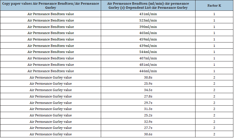
The data of the first two columns of Table 1 were plotted and a linear relation of the two air permeances was revealed. Before performing the ANOVA test, we checked to ensure that our data in Table 1 was normally distributed. The two tests of normality, namely the Kolmogorov-Smirnov test, and the Shapiro-Wilk test were the most widely used methods to test the normality of our data (Figure 1).

Figure 1:Graph of air permeance Gurley in (s) versus air permeance Bendtsen in (ml/min) from the data in Table 1, showed their linear relation.

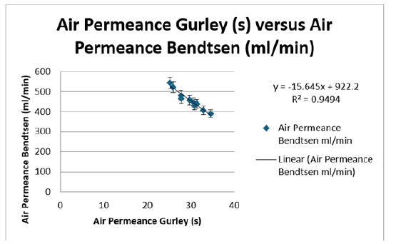
Table 1:Data of the ANOVA, showing the air permeance Bendtsen in ml/min and air permeance Gurley in s/100ml air, of the 100gsm A4 copy paper sample Fabriano. This table was used for presenting the dependent parameter in performing one-way ANOVA, and Factor K.

In Table 2 the quantity Sig.(significance) was the probability of making a mistake if we have accepted that the sample data did not follow the normal distribution. In general, when the sig. was greater than 0.05, we accepted that the distribution was normal. So, in the sample data we have examined the values followed the normal distribution given that sig. (Kolmogorov-Smirnov) =0.2 and sig. (Shapiro-Wilk) =0.805 applied [8].

Table 2:Tests of Normality of data.

In Table 3 we observed that the statistical test of dispersions with the Levene criterion gave the value p=0.002<0.05 which showed that Ho, the null hypothesis was rejected, and that there was no equality of variances for the two groups of data in Table 1, namely air permeance Bendtsen and air permeance Gurley [9].

Table 3:Test of Homogeneity of the variances

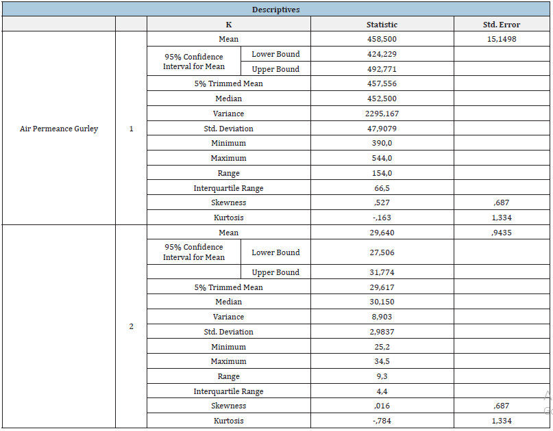
From the Table 4 descriptives it was shown that the median for group 1, air permeance Bendtsen was Q₂=452.5ml/min, the second quartile, and the IQR=66.5ml/min and also the median for group 2, air permeance Gurley was Q₂=30.150s, and the IQR (Interquartile Range) was 4.4s. Also, the skewness value of 0.527 for group 1 was positive indicating a tail to the right of our distribution of data and the kurtosis value below 1, i.e. -0.163, indicated a flat distribution. The skewness value of group 2 was also positive, i.e. 0.016, indicating a tail to the right, and the kurtosis value was -0.784, below 1 indicated also a flat distribution. Comparing though the mean value with the median value for group 1 data, i.e. 458.5ml/ min> 452.5ml/min we concluded that the distribution was skewed to the right, while the mean value was smaller than the median, i.e. 29.640s<30.150s for group 2 data, and the distribution was skewed to the left.

Table 4:Results of Descriptive Statistics [10].

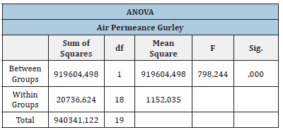
In Table 5 the p-value of ANOVA p=0.000<0.05 applied. The value was close to 0, which indicated that the observed difference was unlikely to have been to chance. That meant at a significant level of α=0.05 there were statistically significant differences between the air permeances values of the two methods Bendtsen and Gurley of Table 1 [11]. Also, F(0.05, 1,18)=798.244>4.4139. Here the F statistic [12] was larger than the critical F-value and the observed differences among the sample means could not reasonably be due to random chance alone. There was insufficient evidence to suggest that the two populations came from the same population of scores. We accepted that the two groups’ variances were significantly different [12]. The result was statistically significant and we rejected the null hypothesis that the means of the two groups of data, air permeance Bendtsen and air permeance Gurley were equal.

Table 5:ANOVA table.

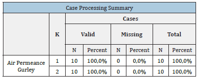
In Table 6 the column valid referred to the non-missing cases of the data in Table 1, which were 10 for both groups of data. In the column missing there was the number of missing cases which was 0. The column total contained the total number of cases in the data set.

Table 6:The Case processing summary.

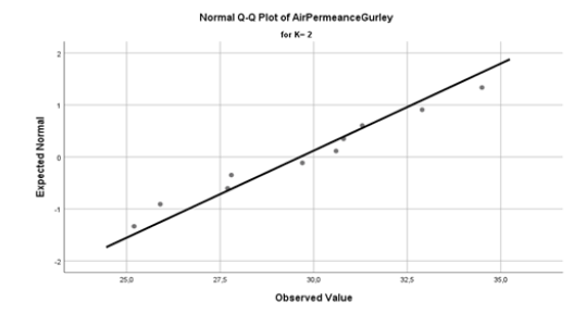
The normal Q-Q (Quantile-Quantile) plots in Figures 2 and 3 compared the observed quantiles of the data of air permeance Bendtsen and air permeance Gurley respectively, depicted as dots, with the quantiles that we would have expected to see if our data of Table 1 were normally distributed (depicted as a solid line) [13]. The Q-Q plots (quantile-quantile) plots were probability plots. That kind of probability plot plotted the quantiles of our variable’s distribution against the quantiles of a test distribution. Our data for air permeance Bendtsen (Figure 2) K=1, and for air permeance Gurley (Figure 3) K=2, were approximately normally distributed, since the points were close to the line. But still when we looked at a Q-Q plot we looked also for points that strayed far from the lines of expected values. Then the Detrended Normal Q-Q Plots were produced.

Figure 2:Q-Q plot for the check of normal distribution for the values of Air Permeance Bendtsen, K=1.

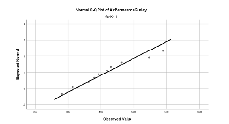
Figure 3:Q-Q plot for the check of normal distribution for the values of Air Permeance Gurley, K=2. Then the Detrended Normal Q-Q Plots were produced.

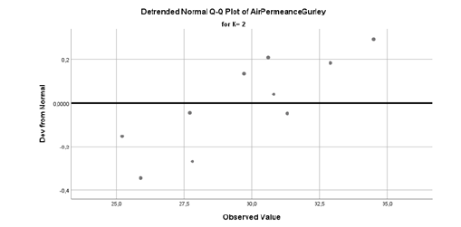
The detrended normal Q-Q plots in Figures 4 and 5 showed the same information as the normal Q-Q plots but in a different manner [14]. In the detrended plot the horizontal line at the origin represented the quantiles that we would have expected to see if our data were normal. The dots in Figures 4 and 5 represented the magnitude and direction of deviation in the observed quantiles.

Each dot was calculated by subtracting the expected quantiles from the observed quantiles. That assumption implied that the dots which were below the trend line on the normal Q-Q plots, appeared above the trend line on the detrended normal Q-Q plot, since observed-expected>0.

Figure 4:Detrended normal Q-Q plot for the check of normal distribution for the values of air permeance Bendtsen, K=1.

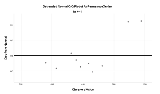
Figure 5:Detrended normal Q-Q plot for the check of normal distribution for the values of air permeance Gurley, K=2.

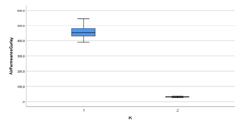
In addition to the hypothesis tests and the quantile-quantile plots of the data of Table 1 we looked at a boxplot of our two groups of data. The boxplots in Figure 6 gave us a better look at the outliers and the location of our quantiles, of our two groups of data [15]. The boxplots of the two samples of our observations 1 and 2, showed the quartiles Q1, Q2, and Q3 with the help of a vertically oriented rectangle. It also showed their extreme values as in group 1 of data of Figure 6. The bottom side of the rectangle of our first group of data (i.e. air permeance Bendtsen), was at the height of the first quartile Q1 and the top side was at the height of the third quartile Q3, and the intermediate parallel corresponded to the median of the sample group Q2. Because the median Q₂=452.5ml/ min divided approximately the rectangle of group 1 into two equal parts we assumed that its distribution was symmetrical. The box plot of group 1 also included two lines outside the rectangle. The first extended from Q1 to Q1-1.5IQR, where IQR=Q3-Q1=66.5ml/ min which was the interquartile range. The observations for group 1 of our data, in Figure 6, that were between 1.5IQR and 3IQR from the upper and the lower side of the boxplot were considered as external outliers.

Figure 6:Boxplot of our two groups of data of Table 1.

The Bendtsen air permeance measurements, and the Gurley air permeance measurements, in Table 1, were evaluated also in (μm/Pa.s) units, [16] according to equations (2) and (3) and were presented in Table 7. In Table 8 there was the case processing summary with the valid, i.e. non-missing cases, the missing cases which were 0 and the total cases which were 10.

Table 7:Data of the ANOVA, showing the air permeance Bendtsen in μm/Pa.s and air permeance Gurley in μm/Pa.s, of the 100gsm A4 copy paper sample Fabriano. This table was used for presenting the dependent parameter in performing one-way ANOVA, and the Factor M.

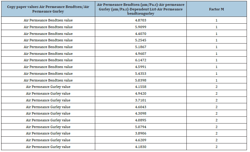
Table 8:The case processing summary.

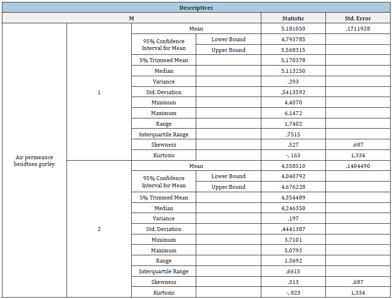
Table 9 the descriptives table showed the summary statistics for each of the two groups of data in Table 7, and in this table all statistics were in the same physical units as the variables in Table 7 that were in μm/Pa.s. The median for group 1 of the data in Table 7 was Q₂=5.113250μm/Pa.s for air permeance Bendtsen and the IQR was 0.7515μm/Pa.s. The skewness and kurtosis values were the same as in Table 4. The median value for group 2 of the data in Table 7 was Q₂=4.246350μm/Pa.s for the values of air permeance Gurley and the IQR was 0.6615μm/Pa.s. The skewness value for group 2 was positive, i.e. 0.313, indicating a tail to the right of the data distribution and the kurtosis value was -0.823 indicating a flat distribution.

Table 9:The Descriptives table.

In Table 10 the sample data of Table 7 followed the normal distribution given that sig. (Kolmogorov-Smirnov)=0.2, and sig. (Shapiro-Wilk)=0.805.

Table 10:The Tests of Normality.

The boxplots in Figure 7 gave us a new look at the outliers and the location of quantiles of both groups of data 1, and 2 of Table 7. The mean value was 5.181050μm/(Pa.s) for group 1 of air permeance Bendtsen, and the mean value was 4.358510μm/(Pa.s) for group 2 of air permeance Gurley, respectively. The median value Q2 was 5.113250μm/(Pa.s) for air permeance Bendtsen, and the median value Q2 was 4.246350μm/(Pa.s) for air permeance Gurley, which were the thick black horizontal lines respectively, inside the two boxplots. The two medians divided each of the distributions into two halves with equal probabilities. Because the median for the group 1 of our data divided the rectangle into two equal parts we assumed that its distribution was symmetrical, unlikely with the data of group 2 which indicated a non-symmetrical distribution.

Figure 7:The boxplots for the two groups of data of Table 7.

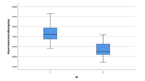
Table 11 included the sizes of the two groups of data, the mean values, the standard deviations and the 95% confidence intervals for means [17]. The lower bound was the value that was less than or equal to every element of the set of data. Upper bound was a value that was greater than or equal to every element of the set of our two groups of data. Because those confidence intervals did not contain zero, we concluded that for level of importance α=0.05 from these data that there was a difference of the means of our two groups of data [18] and that the mean of group 1 was greater than the mean of group 2.

Table 11:The Descriptives Table.

In Table 12 we had the results of equality of variances check. We observed that the statistical test of dispersions with the Levene criterion gave the value p=0.738>0.05 which showed that the null hypothesis was not rejected, i.e. equality of variances, and so ANOVA could be applied, in contrast to the results in Table 3. Because the p-value was large in relation to the α=0.05 value, that meant that statistically we accepted the null hypothesis [19].

Table 12:Results of equality of variances check.

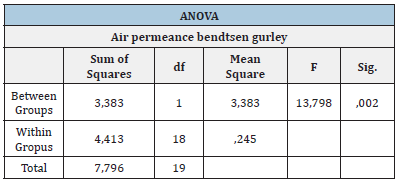
We noticed in Table 13 that for the p-value of ANOVA p=0.002<0.05 applied. Thus, at a significance level of α=0.05 there were statistically significant differences between the values of the two air permeances [20] of the A4 copy paper sample from Table 13. Also, F-test(0.05, 1,18)=13.798>4.4139 and we could conclude that there was at least one parameter value that was nonzero and that the two groups variances were significantly different.

Table 13:ANOVA table.

We attempted to relate the paper property of air permeance according to Bendtsen and according to Gurley. We examined the normality of the values of the two air permeances and we found that they followed the normal distribution given that sig.(Kolmogorov- Smirnov)=0.2 and sig.(Shapiro-Wilk)=0.895. When the two air permeances were expressed in unit’s ml/min for air permeance Bendtsen and in s/100ml air for air permeance Gurley we did not observe equality of variances with the Levene Statistic, i.e. p=0.002<0.05. For the p-value=0.000<0.05 of ANOVA we concluded that there were statistically significant differences between the air permeances of the two methods. From the normal Q-Q plots we obtained that our data for air permeance Bendtsen and Gurley were approximately normally distributed since the points were close to the line.

When the two air permeances were both evaluated in μm/Pa.s units we observed that the sample data followed the normal distribution. We obtained equality of variances with the Levene criterion i.e. p=0.738>0.05 and the null hypothesis was not rejected. For the p-value of ANOVA p=0.002<0.05 and there were also statistically significant differences between the values of the two air permeances of the A4 copy paper sample.

In this work we tried to relate the values of the air permeances according to Bendtsen and according to Gurley but we found that there were statistically significant differences between the two permeances. That conclusion was produced after the one-way ANOVA was applied which was used to check the variability of group means. It was found that the means were not equal and the null hypothesis was rejected. It seemed that the mean value of air permeance Bendtsen did not affect directly the mean value of air permeance Gurley of the copy paper sample tested. It appeared that Bendtsen air permeance was producing different results from measuring Gurley air resistance. The Gurley method may have been only considering penetrating pores with regard to gas transport, but the Bendtsen method may have included also the closed pores and measured the total pore volume of the paper sample.

1. Christer F (2009) Paper products physics and technology. Pulp and Paper Chemistry and Technology 4: 25-67.
2. Yang Y (2014) Effect of changes in fibres’ internal and external fibrillation on dewatering properties in paper making. Master’s thesis for the degree of Master of Science in Technology.
3. ISO 5636-5 (2003) Paper and board-Determination of air permeance and air resistance (medium range)-Part 5: Gurley method.
4. Tarres Q, Aguado R, Pelach MA, Mutje P, Aguilar MD (20220 Electrospray deposition of cellulose nanofibers on paper: Overcoming the limitations of convetional coating. Nanomaterials 12(1): 79.
5. ISO 5636-3 (2013) Paper and board-Determination of air permeance (medium range)-Part 3: Bendtsen method.
6. ISO 187 (2022) Paper, board and pulps-standard atmosphere for conditioning and testing and procedure for monitoring the atmosphere and conditioning of samples, pp. 1-7.
7. Fillat U, Vergara P, Villar JC, Gomez N (2023) Structural properties of coated papers with cellulosic nanofibers using different metering systems and drying technologies. Progress in Organic Coatings 179: 107543.
8. Yusal MS, Bahar I, Namul B (2022) The effect of picture and picture learning model on learning outcomes of junior high school madani makassar students. Bioedupat: Pattimura Journal of Biology and Learning 2(1): 27-31.
9. Gastwirth JL, Gel YR, Miao W (2009) The impact of levene’s test of equality of variances on statistical theory and practice. Statistical Science 24(3): 343-360.
10. Larson MG (2006) Descriptive statistics and graphical displays. Circulation 114: 76-81.
11. Dahiru T (2008) P-value, a true test of statistical significance? A cautionary note. Ann Ib Postgrad Med 6(1): 21-26.
12. Beuckelaer AD (1996) A closer examination on some parametric alternatives to the ANOVA F-test. Statistical Papers 37: 291-305.
13. Liang KK, Ahad NA (2020) Normality for non-normal distributions. JSML 8(2): 51-60.
14. Loy S, Follett L, Hofmann H (2016) Variations of Q-Q plots-the power of our eyes. Am Stat 70(2): 202-214.
15. Schwertman NC, Owens MA, Adnan R (2004) A simple more general boxplot method for identifying outliers. Computational Statistics & Data Analysis 47(1): 165-174.
16. Fernandes SC, Freire CS, Silvestre AJ, Neto CP, Gandini A, et al. (2009) A study of the distribution of chitosan onto and within a paper sheet using a fluorescent chitosan derivative. Carbohydrate Polymers 78(4): 760-766.
17. Bishara AJ, Hittner JB (2017) Confidence intervals for correlations when data are not normal. Behav Res Methods 49(1): 294-309.
18. Geoff C, Finch S (2005) Inference by eye: Confidence intervals and how to read pictures of data. Am Psychol 60(2): 170-180.
19. Greenland S, Senn SJ, Rothman KJ, Carlin JB, Poole C, et al. (2016) Statistical tests, pvalues, confidence intervals and power: A guide to misinterpretations. Eur J Epidemiol 31(4): 337-350.
20. Rendon MY, Scholz MB, Bragagnolo N (2018) Physical characteristics of the paper filter and low cafestol content filter coffee brews. Food Res Int 108: 280-285.