A Statistical Study of the Measurements of the Bekk Smoothness as well as Ash on Ignition and pH Value, of a 100gsm A4 Photocopy Paper

The topography of the paper surface is described using Bekk smoothness and roughness Bendtsen. Apart from them it is described using profile measurements like laser scanning [1- 3]. The Bekk smoothness determined according to ISO 5627 at a defined pressure difference, is the time in seconds in which a specified amount of air required to flow radially inwards between the paper surface and a ring-shaped glass plate, and on into a vacuum chamber [4,5]. The value for the volume of air is for the large vacuum container and a vacuum drop from 50.7kPa to 48.0kPa, i.e. 10.0ml±0.2ml. A drop in the vacuum from 50.7kPa to 48.0kPa means that 10ml of the ambient air has entered the large container.

Alkaline papermaking [6] could be defined as where the wet end pH was above 8 [7]. Although some papermaking additives may have been somewhat alkaline, the quantities used are usually insufficient to enter the alkaline papermaking region. The exception is the addition of calcium carbonate filler, which could take the alkalinity into the range 8-8.5. There is perhaps only one reason for positively managing an alkaline wet end pH, which was to enhance the efficiency of the alkyl ketene dimer (AKD) sizes through the addition of sodium carbonate [8].

The residue (ash content) on ignition at 900oC is related to the content of mineral constituents in the paper sample [5]. For coated and filled products the amount of added mineral constituents could only be calculated from the result if the loss on ignition of the particular pigment used is known. The determination is used as a screening test for checking the overall quality of the copy paper sample. Cellulosic and organic materials as well as carbonate in the sample are completely lost by ignition at 900 °C.

Apart from the analytical methods for paper samples, and surface properties, like smoothness and roughness of the paper there are also the sum parameters which are of special importance [9]. These include the ash content on ignition at 900 °C, pH, and electrical conductivity, of aqueous extracts. In this work, in an attempt to relate the surface property of smoothness Bekk of the paper sample to its inorganic fillers contained in the paper [10] as well as to its pH value we used analysis of variance (ANOVA) [11]. The purpose of this study was to investigate, using statistics, how the surface smoothness of a copy paper sample, which was coated, was affected by the pH value and the ash content on ignition at 900 °C value of the paper sample.

Instruments and materials

The Bekk–Smoothness tester, Frank Prufgerate GmbH Mod.: 33512.F000, S.N. 41454, with power connection 230V/50-60Hz, fuse:3.15AT, power output: 60VA, year of manufacture:10/2006, was used for measuring the Bekk smoothness [4] of the A4 100gsm Multi-paper Fabriano, copy paper sample. The machine measured the paper test pieces of dimensions 100mmx100mm. Ten paper test pieces were measured from side A and ten paper test pieces were measured from side B. The machine was connected with a printer hp. A guillotine IDEAL 1043 GS made in Germany was used for cutting the paper test pieces to dimensions of 100mmx100mm.

A conditioning chamber that was capable of providing and maintaining standard conditions of temperature and humidity, where the paper test pieces were pre-conditioned at 23 °C ± 2 °C and 30%r.h.±5%r.h. for 24hours and were conditioned at 23 °C ± 1 °C and 50%r.h.±2%r.h for 16hours. The paper samples were conditioned for 16 hours at 23±1 °C temperature and 50%±2% relative humidity in accordance with the ISO 187 standard [12] and were tested in the same conditioning atmosphere.

The pH value of the copy paper sample was determined using a Metrohm 716 DMS Titrino, Swiss made, pH-meter and corresponded to the equilibrium pH for 2g of the paper sample dispersed in 100ml of water at a temperature between 20 °C and 25 °C (298K) [13]. The measurement was performed in duplicate and the average value was reported.

For the residue on ignition method the principle required weighing the copy paper sample test pieces in two heat-resistant crucibles of 50ml capacity and igniting both of them at 900 °C in an oven Carbolite England OAF 11/1, maximum temperature 1100 C, S.N. 9/99/2080. The ash mass was determined by weighing the crucible with content after the paper sample had been ignited for 1 hour in the oven. The European reference test method used to determine the ash content on ignition at 900 °C was ISO 2144 [14].

IBM SPSS data analysis software was used throughout this study.

Bekk smoothness was dependent on the shape, the total volume and distribution of the hollow spaces between the surface of the A4 copy paper test pieces, with dimensions 10cmx10cm, and a theoretically ideal plane under the specified conditions of contact [4]. The greater the Bekk smoothness number, the smoother the paper sample. The determination of the pH-value of the copy paper sample was defined by the electrolytes extractable by cold water from the sample of paper. The principle of the method was extraction of the sample of the copy paper of 2g for 1hour with 100ml of cold water of high purity. Then followed filtration of the extract and addition of a salt solution 2ml of 1MKCl. The measurement of the pH value of the extract was performed in duplicate at a temperature between 20 °C and 25 °C [13] and the mean value was calculated to be pH 8.80. The magnitude of the ash content on ignition at 900 °C was related to the content of mineral constituents in the A4 copy paper sample. The determination was performed in duplicate and was used as a test for checking the overall quality of the A4 copy paper product [14].

Comparison of the means of the smoothness Bekk of the two paper sides using One-Way ANOVA (Table 1)

Before performing the ANOVA test, we checked to ensure that our data satisfied the assumption first that our data was normally distributed and second that the variances between the two groups of data (1=side A Bekk smoothness, 2=side B Bekk smoothness) were equal [15]. We first checked the normality of the values of the Bekk smoothness variable of side A and B as was shown in Table 2. From the results, Table 3 of Tests of Normality was very interesting as well as the Q-Q diagram given in the Figure 1. In Table 2 the quantity Sig. (significance) was the probability of making a mistake if we have accepted that the sample data of Table 1 did not follow the normal distribution. The quantity Sig. was greater than 0.05 and we accepted that the distribution was normal. Therefore, in the sample we are considering the values followed the normal distribution given that Sig.(Kolmogorov-Smirnov)=0.200 [16] for both sides of the paper sample and Sig.(Shapiro-Wilk)=0.622 for side A, and Sig.(Shapiro-Wilk)=0.967 [17] for side B (Table 2).

Table 1:Data of the ANOVA, showing the smoothness Bekk in s from side A and side B of the 100gsm A4 copy paper sample Multipaper Fabriano. This table was used for presenting the dependent parameter in performing one-way ANOVA, and the Factor RR.

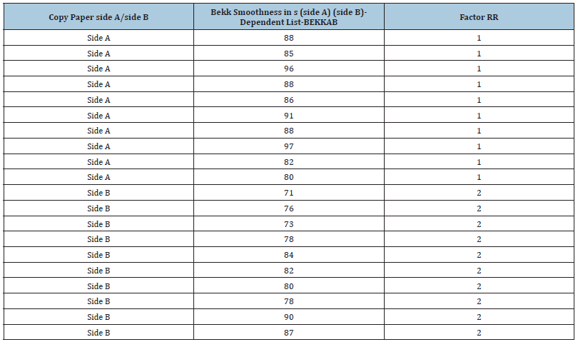
Table 2:Normality check results between groups for smoothness Bekk of the two sides of the A4 100gsm copy paper sample Multi-paper Fabriano. These were the results of the normality check.

Table 3:Homogeneity of dispersion test results and comparison results between groups for smoothness Bekk of the two sides of the A4 100gsm copy paper sample Multi-paper Fabriano. These were the results of equality of variances check.

Figure 1:Q-Q plot for the check of normal distribution.

The tests of normality table provided the results of two tests: a Kolmogorov-Smirnov statistic with a Lilliefors significance correction and a Shapiro-Wilk statistic. A limitation of the Kolmogorov-Smirnov test of normality without the Lilliefors correction was that it would have been very conservative and it would be sensitive to extremes values that would cause tails in the distribution. The Lilliefors significance correction made the test a little less conservative. The Shapiro-Wilk test had more statistical power to detect a non-normal distribution than the Kolmogorov- Smirnov test. The Shapiro-Wilk test was often used when the sample size was less than 50 but could also be used with larger sample sizes. The Shapiro-Wilk test was based on the correlation between the data and the corresponding normal scores. The values of the Shapiro-Wilk statistic usually ranged between zero, which indicated non-normality of the data, and a value of one which indicated normality. A distribution that passed those tests of normality provided extreme confidence that the parametric tests could be used [17,18].

The same conclusion of normality was also obtained from the normal Q-Q (quartile-quartile) plot of Figure 1. In order for the sample to be normal in that diagram all the points should have been on the straight line. We noticed from Figure 1 that that was true for the variable we examined, i.e. the Bekk smoothness values of both sides of the copy paper sample [19]. For both the Shapiro-Wilk and Kolmogorov-Smirnov tests, the p-value greater than 0.05 provided evidence that the distribution was significantly normal. These both tests of normality did not provide information about why a variable was normally distributed and therefore was important to obtain skewness and kurtosis values in order to inspect the distribution of data and identify any reasons for non-normality as it was presented in Table 4.

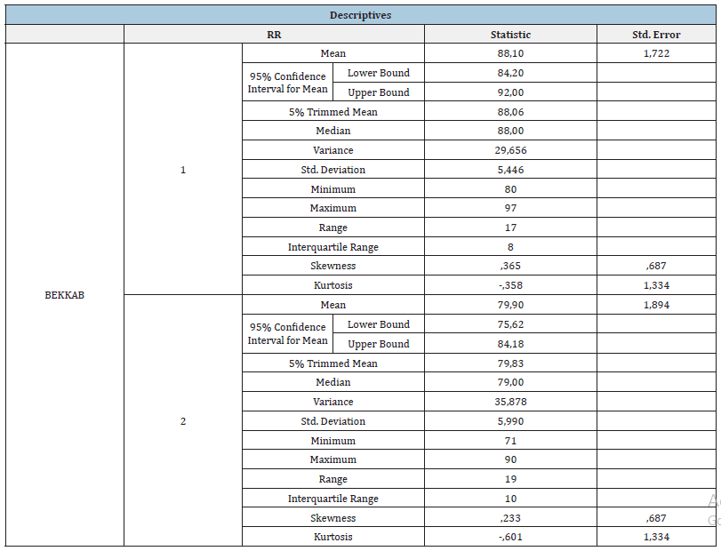
Table 4:Descriptives Table.

From the above Table 3, Test of Homogeneity of variances, we observed that the statistical test of dispersions with the Levene criterion [20] gave the value p=0.628>0.05 which showed that Ho, the null hypothesis, was not rejected, i.e. equality of variances. Consequently, there was no statistically significant difference in the dispersion of the Bekk smoothness of the two sides of the A4 copy paper sample, and so ANOVA could be applied. We also noticed that for the p-value of ANOVA p=0.005<0.05 applied (Table 5). Thus, at a significance level of a=0.05 there were statistically significant differences between the Bekk smoothness values of the two sides of the A4 copy paper sample, and thus the null hypothesis was rejected.

Table 5:Analysis of Variance (ANOVA).

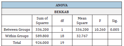
From Table 5 seemed that in level of significance a=0.05 but also at significance level a=0.01 there were statistically significant differences between the smoothness Bekk values of the two sides A and B (p=0.005<0.01). ANOVA was concerned with the testing of hypotheses about means and it was very similar to a t-test. In fact, for this experiment, involving two groups, the output from ANOVA and t-test would be the same. However, the t-test could not be used to test hypothesis on three or more groups and then ANOVA would be used. The one-way Analysis of variance (ANOVA) using an F-test of difference in mean value of Bekk smoothness side A against mean value of side B determined if the mean values differed significantly. The method of analysis was dependent upon Levene’s test of homogeneity of variances, a procedure designed to test the null hypothesis all group variances were equal. The Levene output p-value was 0.628 greater than 0.05, and equal variances could be assumed and standard ANOVA procedure could be carried out using Tukey’s HSD post-hoc analysis [21]. From Table 5 the F-test was used in regression analysis to test the hypothesis that all model parameters were zero. Since F=10.260>3.00 we could conclude that there was at least one parameter value that was nonzero. The F statistic was larger than 3.00 then the result was significant (p<0.05), F(2, ∞)=3.00<10.260.

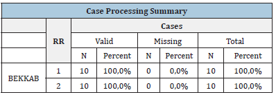
In Table 6, in the case processing summary, the column valid referred to the non-missing cases. In that column valid the N was given, which was the number of non-missing cases; and the percent was given, which was the percent of non-missing cases. Missing referred to the missing cases. In that column the N was given, which was the number of missing cases; and the percent was given, which was the percent of the missing cases. The total referred to the total number cases, both non-missing and missing. In that column the N was given, which was the total number of cases in the data set; and the percent was given, which was the total percent of cases in the data set [22].

Table 6:

The Table 4, below, the descriptives table showed the summary statistics for each of the two variables Bekk smoothness side A and side B. In the table all statistics were in the same units as the original variables that was in seconds. The exceptions were the variance, which was in squared units and the skewness and kurtosis values, which were in units that were relative to the normal distribution. From the descriptives table we obtained further information about the distribution of the variable. A perfectly standard normal distribution had skewness and kurtosis values equal to zero. The skewness value was positive which indicated a tail to the right. The descriptives table showed that the skewness values for Bekk smoothness were between -1 and +1 suggesting that the distributions of these variables were within the limits of a normal distribution. The kurtosis value below 1 indicated that the distribution tended to be flat [19].

In Table 4 the Descriptives table was a procedure to summarize the continuous data. The descriptive statistics also provided different statistics; one was the distribution of score on continuous variables like skewness and kurtosis. Those statistics were important before we used the parametric statistical technique ANOVA. In the descriptives table the mean was the arithmetic mean across the observations. It was a measure of the central tendency. It was the commonly called average. The mean was sensitive to extremely large or small values. The 95% confidence interval for mean lower bound was the lower (95%) confidence limit for the mean. It gave some idea about the variability of the estimate of the true population mean. The 95% confidence interval for mean upper bound was the upper (95%) confidence limit for the mean. The 5% trimmed mean was the mean that was obtained when the lower and upper 5% of values of the variable were deleted. Because the value of the 5% trimmed mean, i.e. 88.06s, was not very different from the mean, i.e. 88.10s, that indicated that there were not any outliers present. However, we could not assume that all outliers have been removed from the trimmed mean.

In the same Table 4, the median i.e. 88.00s splitted the distribution such that half of all values were above that value and half were below. The variance was a measure of variability. It was the sum of the squared distances of a data value from the mean divided by the variance divisor. The variance was the corrected SS value divided by N-1=9. The corrected SS value was the sum of squared distances of a data value from the mean. The range was a measure of the spread of the variable, here the Bekk smoothness value of the copy paper sample. In the Table 4 the interquartile range was the difference between the upper and the lower quartiles. It measured the spread of the set of our data and was robust to extreme observations. The skewness measured the degree and direction of asymmetry, i.e. provided indication if the distribution was symmetric or not. Kurtosis was a measure of the heaviness of the tails of the distribution and provided information about the peakedness of our distribution. The kurtosis value -0.358 was negative because the tails were lighter than for a normal distribution. The kurtosis was a measure of tail extremity reflecting either the presence of outliers in our distribution or our distribution’s propensity for producing outliers [23]. Of course, if our distribution was perfectly normal, we would have had a skewness and kurtosis value of 0. The positive skewness value of 0.365 for the side 1 of the paper sample indicated positive skew which meant that the scores clustered at the low values of the scale and there were very few higher scores. That happened because the mean was higher than the median value, i.e. 88.10s>88.00s. Our data may have been considered to be approximately normal in shape, since the skewness was 0.365 and kurtosis was –0.358, and both were between -1.0 and +1.0 for side 1 of the Bekk smoothness value of our copy paper sample, as well for side 2, where skewness was 0.233 and kutrosis was -0.601.

A robust regression methodology was presented in Table 7 via M-estimation. Robust regression analysis was used in order to analyse data containing outliers. The approach adapted to the tail behavior and skewness of the distribution of the random error terms, providing for a reliable analysis under a broad class of distributions [24]. In Table 7, we were given also the weighting constants for the weighting functions for the method M-estimator with Huber’s and, Tukey’s biweight function, as well as Hampel’s and Andrews’ wave. The percentile method of determining normal limits was discussed. The primary advantage of that method was that the reliability of sample percentiles could be determined without making any assumptions about the distribution shape, like Guassian or other of the population from which the sample was drawn [25].

Table 7:M-Estimators.

In the above Table 8, of percentiles we had the weighted average, and those were the percentiles for the variable Bekk smoothness side A and side B. If there were not a value at exactly the 5th percentile then the value would be interpolated, which was not the case here. The Tukey’s Hinges were the first, second and third quartile. They were calculated the way that Tukey originally proposed when he came up with the idea of the boxplot. The values were not interpolated; rather they were approximations that could be obtained with little calculation. The 25 was the 25% percentile, also known as the first quartile and was 85.00 and also 76.00. The 50 was the 50% percentile, the second quartile, also known as the median and was 88.00 and 79.00. It was a measure of the central tendency. It was the middle number when the values were arranged in ascending or descending order. The median was a better measure of central tendency than the mean, because it was less sensitive than the mean to extreme observations. The 75 was the 75% percentile, also known as the third quartile, and was 91.00 and 84.00.

Table 8:Percentiles.

Table 9:Extreme values

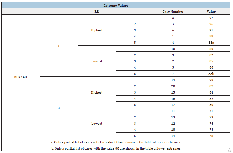
In the extreme values Table 9, above, the five largest and five smallest values of the two variables, Bekk smoothness of paper side A and side B and the corresponding case numbers or data base rows were obtained and were shown [19]. It was important to identify outliers and extreme values that caused skewness. However, the values in the Extreme values table were the minimum and maximum values in the data set, and those may not have been influential outliers. The table of extreme values gave the upper and lower extremes. The outlier or extreme value was defined as the data point that deviated from the other observations, that it became suspicious to be generated by a totally different mechanism or simply by error. Identifying outliers was important because those extreme values could increase the error variance of our data.

Comparison of the means of the smoothness Bekk of the two copy paper sides and also of the ash on ignition content values and pH values of the paper sample, using One-Way ANOVA and Post-Hoc tests

In order to see if there were differences or relations between the properties of the paper sample such as smoothness Bekk values on both sides of the paper, as well as the values of ash on ignition at 900 °C and the pH values, we constructed Table 10 with those data, for the A4 copy paper sample, and we applied ANOVA and we did the Post Hoc Tests and we chose the Tukey test, since we had homogeneity of the dispersion. In the results we got also the Tables 11 & 12 and the tables for the post-hoc tests.

Table 10:ANOVA table with data and, also data for the Post-Hoc Tests, showing the smoothness Bekk in s from side A and side B of the 100gsm A4 copy paper sample Multi-paper Fabriano, as well as the values of ash on ignition at 900 °C, in %w/w, and the values of pH. This table was used for presenting the dependent parameter in performing ANOVA and Post-Hoc Tests, and Tukey, and the Factor TT.

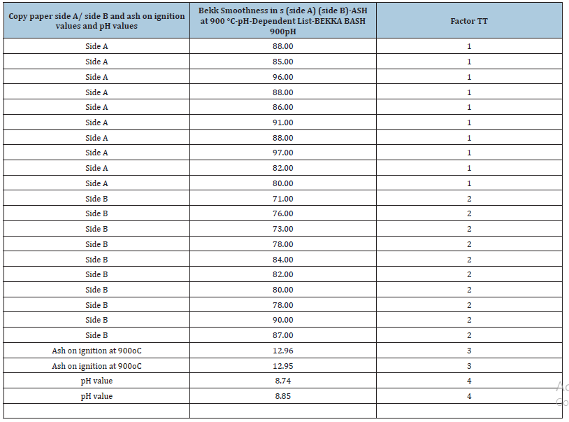
Table 11:Homogeneity of dispersion test results and comparison results between groups for smoothness Bekk of the two sides of the A4 copy paper as well as between the ash on ignition value and pH value of the copy paper.

Table 12:ANOVA table with data

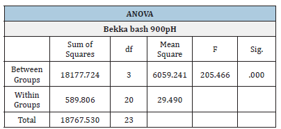
From the above Table 11, test of Homogeneity of variances we observed that the statistical test of dispersions with the Levene criterion gave the value p=0.146>0.05 which showed that Ho, the null hypothesis was not rejected. Consequently, there was no statistically significant difference in the dispersion of the Bekk smoothness of the two sides of the paper as well as of the values of ash on ignition and the values of pH, and so ANOVA could be applied. We also noticed that for the p-value of ANOVA p=0.000<0.05 applied (Table 12). It was necessary before performing the ANOVA test to check and ensure that our data satisfied the two assumptions of a normal distribution and that their variances between the groups were equal.

The Post-hoc analysis performed in Table 13, offered more insight into discrepancies or similarities between the particular groups of data considered in this study and was thus an essential step in the analysis of data [26].

Table 13:Results of partial comparisons. Some post hoc tests were reported in multiple comparison tables. *The mean difference is significant at the 0.05 level.

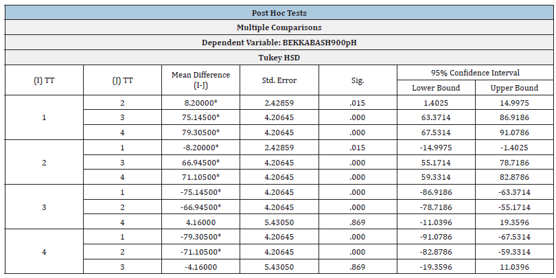
From Table 13, for the group 1 versus group 2 [mean difference=8.20000, p=0.015(<0.05)]; this indicated that there was a significant difference at the 5% level between the mean of the group 1 (mean=88.03s) compared to the mean of group 2 (mean=79.82s). Similarly, for the group 1 versus group 3 [mean difference=75.145, p=0.000(<0.05); this indicated that there was a significant difference at the 5% level of significance between the mean of the group 1 Bekk smoothness (mean=88.03s) compared to the mean of group 3 ash on ignition (mean=12.96%w/w/). Similarly, for the group 1, mean 88.03, versus group 4 (mean=pH8.80) p=0.000<0.05; that indicated that there was a significant difference at the 5% level of significance between the mean of the group 1 compared to the mean of group 4. The same applied for group 2 versus group 1, 3 and 4. Also, the same applied for group 3 versus groups 1 and 2. Finally, for the group 3 versus group 4 (mean difference=4.16000, p=0.869(>0.05); indicating that there was no significant difference between the means of the ash residue on ignition and the pH value. Also, for the group 4 versus group 3, (mean difference=-4.16000, p=0.869 (>0.05); indicating that there was no significant difference between the means of the pH value and the ash content on ignition at 900 °C of the copy paper sample.

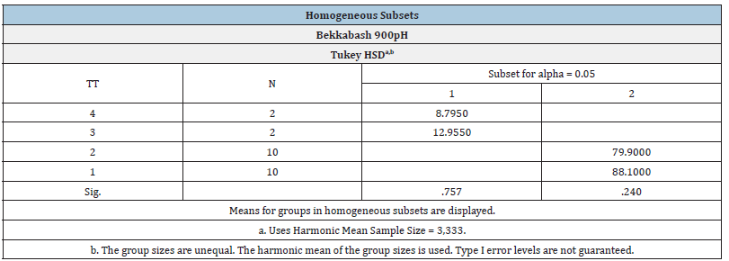
The Homogeneous subsets output was produced by a request for post hoc tests and addressed the same questions as the multiple comparisons table for post hoc analysis, i.e. which pairs of groups had significantly different means on the dependent variable which was Bekk smoothness-ash on ignition and pH. Like the multiple comparisons table, the homogeneous subsets output would not be interpreted if the main effect (ANOVA table) was not significant.

In this study, some post-hoc tests were only reported as homogeneous subset output; some were only reported as multiple comparison tables; and some were reported in both formats, i.e. Tukey HSD, as it was in this study. The homogeneous subsets table showed which groups had the same mean and which of them had different means. Within a subset there was no significant difference while between subsets there was a significant difference (Table 14). The means for groups 4 and 3 appeared in subset 1 while groups 2 and 1 appeared in subset 2. The interpretation was that groups 4 (pH) and 3 (ash on ignition at 900 °C) were significantly different from groups 2 (smoothness Bekk side A) and 1 (smoothness Bekk side B), because groups 4 and 3 never appeared in any subset with either group 2 or 1. The tests available in the multiple comparisons table had better properties than the homogeneous subset tests [30,31] and they were the preferred focus for our post hoc analysis.

Table 14:Results of partial comparisons. Some post hoc tests were reported in Homogeneous subsets [27-29].

We attempted to relate the surface property of smoothness Bekk to the pH value and ash content on ignition at 900 °C. We first examined the normality of the values of the Bekk smoothness of the two sides of the copy paper sample and we accepted that they followed the normal distribution, since sig.(Kolmogorov- Smirnov)=0.2>0.05 and also sig.(Shapiro-Wilk)=0.622>0.05, and sig.(Shapiro-Wilk)=0.967>0.05. The same conclusion of normality was obtained from the normal Q-Q plot. From the test of Homogeneity of variances with the Levene statistic the null hypothesis was not rejected, and we observed equality of variances. For the p-value of ANOVA p=0.005<0.05 and there were statistically significant differences between the Bekk smoothness values of the two sides of the A4 copy paper sample.

We obtained the case processing summary and also the descriptives table for the Bekk smoothness values of the two sides of the paper sample. The descriptives table showed that the skewness value was positive and indicated a tail to the right. We then had the table of percentiles for the variable Bekk smoothness side A and side B, and the extreme values table which provided the five largest and five smallest values of the two variables. We then compared the value of the Bekk smoothness with the value of pH and the value of the ash on ignition. The test of homogeneity of variances was performed before ANOVA. Finally, post hoc tests were reported and in the multiple comparisons table the mean differences indicated that there were significant differences at the 5% level of significance between the means of the groups of Bekk smoothness and the ash on ignition, as well as the pH value of the paper sample. But there was no significant difference between the means of the pH value and ash content on ignition at 900 °C.

The aim of this study was to determine the possibility of relating the ash content value and pH value and to assess how they influence the paper surface property of Bekk smoothness of the copy paper sample. It seemed that the mean values of pH and ash residue did not affect directly the mean value of smoothness property Bekk, of the copy paper. It appeared that the small particles of mineral constituents did not cover the gaps between the fibres of paper, allowing air to pass between them and the alkaline pH value did not enhance that phenomenon. The pH 8.8 value did not influence the embedding of the mineral constituents in the mass of the copy paper and thus they did not affect the physical characteristic of the Bekk smoothness of the copy paper.

1. Chinga G, Gregersen O, Dougherty B (2023) Paper surface characterisation by laser profilometry and image analysis. Microsc Anal 96: 21-23.
2. Ismail MY, Patanen M, Kauppinen S, Kosonen H, Ristolainen M, et al. (2020) Surface analysis of tissue paper using laser scanning confocal microscopy and micro-computed topography. Cellulose 27: 8989-9003.
3. Elgay P (1994) Non-contact laser surface profilometry. UMI, State University of New York College of Environmental Science and Forestry, USA.
4. ISO 5627 (1995) Paper and board-Determination of smoothness (Bekk method), pp. 1-7.
5. Caprita FC, Ene A, Ceoromila AC (2021) Valorification of Ulva rigida algae in pulp and paper industry for improved paper characteristics and wastewater heavy metal filtration. Sustainability 13(19): 10763.
6. Hubbe MA (2004) Acidic and alkaline sizings for printing, writing and drawing papers. The Book and Paper Group Annual 23: 139-151.
7. Mannai F, Ammar M, Yanez JG, Elaloui E, Moussaoui Y (2018) Alkaline delignification of cactus fibres for pulp and papermaking applications. Journal of Polymers and the Environment 26: 798-806.
8. Roberts JC (1997) A review of advances in internal sizing of paper. In the Fundamentals of Papermaking Materials, Trans of the XIth Fund Res Symp Cambridge, Baker CF (Ed.), FRC, Manchester, pp.209-263.
9. Otmar T (2006) Testing of paper and board. Wiley Online Library 467-474.
10. Kim SY, Jung SY, Seo YB, Han JS (2023) Preparation of flexible calcium carbonate by in situ carbonation of the chitin fibrils and its use for producing high loaded paper. Mater 16(8): 2978.
11. Benli M, Gumus BE, Kahraman Y, Yagci O, Erdogan D, et al. (2021) Thermal, structural and morphological characterization of dental polymers for clinical applications. J Prosthodont Res 65(2): 176-185.
12. ISO 187 (2022) Paper, board and pulps-standard atmosphere for conditioning and testing and procedure for monitoring the atmosphere and conditioning of samples, pp.1-7.
13. ISO 6588-1 (2021) Paper, board and pulps-determination of pH of aqueous extracts Part 1: Cold extraction, pp.1-7.
14. ISO 2144 (2019) Paper, board, pulps and cellulose nanomaterials-determination of residue (ash content) on ignition at 900 °C, pp. 1-10.
15. Garson GD (2012) Testing statistical assumptions. (2012 edn), Statistical Associates, Publishing Blue Book Series, USA.
16. Lilliefors HW (1967) On the kolmogorov-smirnov test for normality with mean and variance unknown. Journal of the American Statistical Association 62(318): 399-402.
17. Razali NM, Wah YB (2011) Power comparisons of shapiro-wilk, kolmogorov-smirnov, lilliefors and anderson-darling tests. Journal of Statistical Modeling and Analytics 2(1): 21-33.
18. Marden JI (2004) Positions and QQ plots. Statist Sci 19(4): 606-614.
19. Barton B, Peat J (2014) Medical statistics: A guide to SPSS, data analysis and critical appraisal. (2^nd edn), John Wiley & Sons.
20. Lemeshko BY, Lemeshko SB, Gorbunova AA (2010) General problems of metrology and measurement technique, application and power of criteria for testing the homogeneity of variances, Part I, parametric criteria. Measurement Techniques 53(3): 237-246.
21. Halsell JN (2007) Using cluster analysis to evaluate the academic performance of demographic homogeneous subsets. UNLV Retrospective Theses & Dissertations 2761.
22. Pardo TA, Antiqueira L, Nunes GV, Oliveira ON, Costa LD (2006) Using complex networks for language processing: The case of summary evaluation. International Conference on Communications, Circuits and Systems, Guilin, China, pp. 2678-2682.
23. Westfall PH (2014) Kurtosis as peakedness, 1905-2014. R.I.P. Am Stat 68(3): 191-195.
24. Nahar J, Purwani S (2017) Application of robust M-estimator regression in handling data outliers. 4^th ICRIEMS Proceedings, Published by the Faculty of Mathematics and Natural Sciences, Yogyakarta State University, ISBN 978-602-74529-2-3, pp. M53-M-60.
25. Herrera L (1958) The precision of percentiles in establishing normal limits in medicine. J Lab Clin Med 52(1): 34-42.
26. Ferreira DF (2014) Sisvar: A guide for its bootstrap procedures in multiple comparisons. Cienc Agrotec Lavras 38(2): 109-112.
27. Halsell Jeffrey N (2007) Using cluster analysis to evaluate the academic performance of demographic homogeneous subsets. UNLV Retrospective Theses & Dissertations 1-189.
28. Muogbo PC, Obasa PA (2021) Homogeneous subset stance of rhizome length and operational machine speed on planting parameters of tractor drawn turmeric planter. EPRA IJRD 6(6): 4-10.
29. Ataci N, Sinsek G, Atac IA, Kuzu H (2009) Temperature and pH effect on milk clotting time of mucor miehei rennet. Asian J Chem 21(3): 1754-1758.
30. Gabriel KR (1969) Simultaneous test procedures-some theory of multiple comparisons. Ann Math Stat 40(1): 224-250.
31. Demsar J (2006) Statistical comparisons of classifiers over multiple data sets. Journal of Machine Learning Research 7: 1-30.