
- About Us
- Information
-

The Author ensures that the research has been conducted responsibly and ethically with adherence to all relevant regulations. read more..
- For Authors
- For Reviewer
- Manuscript Guidelines
- Membership
- Publication Ethics
-
- Journals
- Reprints
- e-Books
- Videos
- Policies
- Contact Us
 COVID-19
- Submissions


Full Text
Annals of Chemical Science Research
Role of Cellulose in Determining the Mechanical and Optical Properties of Two Soft Paper Roll Samples and Application in the Mechanics of the System of the Fourth Order Improved Runge-Kutta Method
Chryssou K*, Stassinopoulou M and Lampi E
General Chemical State Laboratory, Greece
*Corresponding author: Chryssou K, General Chemical State Laboratory, Greece
Submission: February 16, 2021Published: February 25, 2021

Volume2 Issue3February, 2021
Abstract
White soft paper sample rolls from Glass Cleaning S.A. were tested for their tensile and optical properties as well as the fibre component of their pulps using the optical microscope. Also, other substrate properties of the two soft paper roll samples were determined i.e., ash content on ignition at 900 °C, brightness, basis weight, the band gap energy, and finally application in the mechanics of the system of the 4th order Runge-Kutta method of two different step sizes was implemented on the two wet paper strips used for determining their wet tensile strength.
Keywords: Cellulose; Optical microscope; Tensile strength; Absorption spectra; Kubelka-Munk K/S value; Band gap energy; Fourth order Runge-Kutta method.
Introduction
In this work a fibre furnish analysis was carried out under the optical microscope to
determine the fibre component of the pulps of two soft paper roll samples quantitatively.
The physico-chemical characteristics of the paper roll sheets were connected to the chemical
composition of the obtained pulps [1]. The Herzberg staining test was applicable to the
qualitative and quantitative differentiation between chemical, mechanical and rag pulps [2-
4]. Here the pulp of the paper samples was identified as chemical, i.e., cellulose.
With the development of micro-electro-mechanical systems technology, more thin
materials have been used in this field. A method is proposed to measure the mechanical
properties of thin sheets of soft paper. The tensile properties of the dry and wet soft paper
samples were carried out using a Zwick-Roell Z.2.5 machine with a 50N load cell [5-7]. The
tensile-testing apparatus stretched the soft paper test pieces strips at a constant rate of
elongation of 50±2mm/min. The paper test specimens strips were conditioned at (23±1) °C
and (50±2)% relative humidity (r.h.) before and during the testing. With the rapid development
of electro-mechanical systems more thin materials including paper and plastics products
have been widely used. The mechanical properties such as tensile strength and elongation at
rupture are necessary for producing soft paper products and plastic products and evaluating
their reliability [6]. Of all the methods proposed to measure the properties of soft paper
products the uniaxial tensile test has been generally considered as the most reliable way. The
difficulty of the uniaxial tensile test is how to fabricate a thin, undamaged, straight, smooth
and with parallel edges strip, align the paper strip, and measure the strain. A micro-tensile
method has been implemented for measuring the mechanical properties of micro-electromechanical
systems materials and measure the strain [6]. The mechanical behavior of paper
samples and polymers is also temperature dependent. Many models have been proposed
for the determination of the relationship between temperature, relative humidity, strength,
stress and strain. The high tensile strength appearing lengthwise for both paper samples rolls
was caused by the grain-boundary strengthening and grain preferred orientation [6]. Also, in
this work a tensile test system was presented to measure the tensile strength of the soft paper
strips in their dry and wet state.
Generally cellulose fibres are used in the production of paper
pulp and they impart mechanical strength properties [8]. In
cellulose, a polymer of glucopyranose units (β-D) linked together
by the association of β-glycosidic bond to be a long chain and
are connected with other hydrogen bond chains [8]. The tensile
strength was calculated using the formula σ=F_max/A (1), where
Fmax was the maximum force and A was the cross-sectional area
of the paper 50mm strip of the two soft paper roll samples [8,9].
The inference from the data from this work was that cellulose
was the key mechanical component contributing to mechanical
strength [9,10]. The mechanical properties of soft paper rolls
mainly depended on the structure and strength of cellulosic fibers
[11,12] which bear the exterior loads. Cellulose was behaving as a
mechanical element. It behaved as a mat of individual fibrils. The
assessment of the cellulosic fiber for the two soft paper samples was
conducted with the determination of strength and strain to failure
using paper strip tensile tests [8,9]. The mean tensile strength and
the standard deviation were calculated also.
The cellulose fibre pulp of the two paper sample rolls in this
work was separated from the other biomass components by
pulping and by the bleaching process [10,11]. Finally, this paper
deals with a special ordinary differential equation. The purpose
of this work was to propose a mathematical model. Fourth order
improved Runge-Kutta method for directly solving a special thirdorder
ordinary differential equation was constructed by Hussain et
al. [13]. Numerical comparisons were performed using the existing
Runge-Kutta method after reducing the problems into a system of
first-order equations and solving them, and direct RKD (Runge-
Kuttta) method for solving special third-order ordinary differential
equations. Numerical examples were presented to illustrate the
efficiency and the accuracy of the method in terms of a number of
function evaluations and the max absolute error. In this work the
4th order Runge-Kutta method of two different step sizes h=0.5 and
h/2=0.25 was implemented for both of two soft paper samples
in the Matlab computing environment. A Runge-Kutta 4th order
method for solving an ordinary differential equation was developed
and implemented [13].
Experimental
Reagents
All the chemicals used were of analytical reagent grade quality and they were used without further purification. Solutions were prepared using deionized water of conductivity <1μS/cm. Zinc chloride for analysis (250g) was procured from M EMSURE (M.W.136.30g/mol). Potassium Iodide for analysis (250g) was procured from M EMSURE (M.W. 166.00g/mol). Iodine, IODIO BISUBLIMATO (100g) was procured from Carlo Erba (Cod. 455959). Calcium chloride anhydrous (M.W. 110.99g/mol) QP desiccant was procured from Panreac (1000g) (Code 211221.1211).
Apparatus
Ordinary laboratory equipment such as beakers of capacity
100ml, and glass cylinders of capacity 100ml were used. The microscope used was a projection optical microscope SDL S.N.,
232431, 220V, 60W, S1, with a round screen and no binoculars,
and with a magnification of x10/0.2 to x20/0.4. The microscope
slides used were of size 25mmx75mm. Rectangular microscope
cover glasses of size 22mmx33mm were also used. An ultra-sonic
disperser was used to prepare the paper fiber suspensions. A
dropper, which was a glass tube of 100mm in length and with an
internal diameter 5mm with one end carefully smoothed and the
other end fitted with a rubber bulb, which discharged 0.5ml of
paper fibre suspension onto the microscope slides.
The tensile strength machine used was a Zwick-Roell Z.
50N with a longstroke extensometer code number 320109.
The tensile testing machine Zwick Roel extended the paper test
pieces of dimensions 50mmx90mm at 50mm/min constant rate
of elongation and measured the maximum tensile force. It had a
strength force of 50N. The tensile testing machine measured the
maximum tensile force to an accuracy of ±1% of the true force.
The machine had an extensometer placed directly on the paper
test piece for the measurement of its elongation. The machine was
connected with a computer LG and was accredited every three
years. The tensile testing machine included two clamps for holding
the paper test pieces of 50mm width. The clamps gripped the test
pieces firmly along a straight line across the full width of the test
piece and adjusted the clamping force pneumatically. The machine
had a pneumatic grip of 2.5kN, and a longstroke extensometer with
code number 320109.
Absorption spectra were obtained also by means of a
Spectrophotometer CM-3630, BCMTS M Type 40605, S.N. 43029,
TouchScreen-M V 2.0, Frank-PTI. The spectrophotometer CM-3630,
Model BCMTS M Type 40605, had a software Touchscreen M. The
apparatus was connected with a computer Asus with windows
7Pro. The computer had a display Hanns. G and a keyboard Logitech
K120, a mouse Logitech RX250, and a printer HP LaserJet P1102.
The spectrophotometer also had a black cavity made in Japan
with a reflectance factor which did not differ from its nominal
value by more than 0.2% at all wavelengths. It also had a white
calibration plate Konica Minolta with number 20286101. It also
used for calibration a paper non-fluorescent reference standard for
adjusting the UV-content of the radiation incident upon the sample
with number CNF-082, and a paper fluorescent reference standard
for adjusting the UV-content of the radiation incident upon the
sample with number CF-082, IR 3 Ctp.
Weighings were carried out on an electronic balance Sartorius
Basicplus, AGGöttingen Germany BP 221S, with maximum capacity
220g, precision of four decimal places, and accuracy to 0.1mg and it
was accreditated every three years. A Bunsen burner with a flame
with a reducing internal cone was used where the dishes with the
paper sample specimens of size approximately 1cmx1cm, were
heated slowly in such a manner that the paper sample specimens
were burned and did not burst into flames. Also, no material was
lost in the form of flying particles. The intensity of the flame was
such that its internal cone was not into contact with the porcelain of the dish. Glass containers were procured from NS ISOLAB Germany,
and were used with a diameter of 80mm, a height of 30mm, and a
capacity of 80ml, inside which the soft paper test pieces were kept
and weighed. A glass desiccator, with a plate from porcelain with
holes, and with CaCl2 as desiccant, was used for the transferring
of the porcelain dishes, inside which were kept the test pieces of
the two soft paper samples, and finally the dishes with the ash
content. Dishes of porcelain with an even bottom with a diameter
of 5cm, a height of 4.5cm, and a capacity of 50ml were used for the
incineration of the paper sample specimens. The dishes did not lose
and did not gain mass on ignition. Before their use the dishes were
rinsed with distilled water and then they were heated at 900 °C±25
°C inside the furnace for 60min. After the passage of two hours their
temperature diminished at 400 °C and the dishes were kept for two
hours into the desiccator before they were used.
A muffle furnace Carbolite of maintaining a temperature of
900 °C was used. The muffle furnace Carbolite type OAF 11/1
S/N 9/99/2080, with max temperature 1100 °C was used, of
maintaining a temperature of 900 °C±25 °C, i.e. 918 °C. It constituted
from thermal plates which made the roof and its floor. The furnace
had a built in pre-heated stream of air which passed through its
chamber. It was also provided with a chimney to evacuate smoke
and steam and fumes. The furnace was accreditated every three
years. A drying oven Memmert GmbH UNE 400 was used, which
maintained air temperature at 105 °C±2 °C and it was ventilated in
order to maintain uniform temperature and extracted the moisture
from the two soft paper test pieces [14] and it was accreditated
every three years. An Oven Memmert direkt, was used capable of
being controlled at 1030C±20C, where the microscope slides with
the paper fiber suspensions on them were heated and dried. The
cutting device used was a guillotine IDEAL 1043 GS DP 02050
made in Germany which produced paper test pieces strips of 50mm
wide and 100mm in length with undamaged, straight smooth and
parallel edges.
An accreditated ruler for measuring the width of the soft paper
test pieces strips and also of measuring the rate of elongation
was used. The metallic ruler was accreditated from an external
accreditated body every five years. The tensile properties of the
soft paper roll samples vary at different temperatures and relative
humidities. Therefore, a conditioning room where the soft paper
samples were conditioned for eighteenteen (18) hours before
testing and tested in a standard atmosphere at (23±1) °C and at
(50±2)% relative humidity was used [15]. The conditioning chamber
provided and maintained standard conditions of temperature and
humidity, where the soft paper test pieces were pre-conditioned at
23 °C±2 °C and 30%r.h.±5% r.h, and were conditioned at 23 °C±1 οC,
and 50%r.h.±2% r.h., and was accreditated each year.
Preparation of herzberg stain
We weighed 50g of ZnCl2 into a 100ml glass beaker and we added 25ml of deionized water. We then weighed 0.25g of I2 and 5.25g of KI into another 100ml glass beaker and we added 12.5ml of deionized water. We then stirred the contents of the two beakers with glass rods until dissolved and we transferred the two solutions to a glass cylinder of 100ml capacity and we stoppered the cylinder. We shaked the cylinder well to mix the solutions and finally left it overnight away from light and air, in the dark, so that the precipitate formed settled. After 24 hours we decanted the clear solution into a brown dropper bottle with a ground-glass stopper and we kept it away from air and light in the dark.
Preparation of the paper fiber suspension
The paper fiber suspensions were prepared in the ultra-sonic disperser by putting the test paper pieces of each of the two soft paper samples, of size approximately 1cmx1cm and adding 400ml deionized water. The paper pulp was homogenized in a Waring commercial blender (mixer) setting low and high for 3 minutes.
Staining and preparation of fibre slides for optical microscopy
We put 1ml of the paper fiber suspension on to the microscope slide and we dried the slide with the suspension onto it, for 10min in the oven Memmert direct controlled at 103 °C±2 °C. As the slide with the suspension was hot from the oven, we stained the fibres of each of the two paper samples by applying 3 drops of the Herzberg stain onto the fibre slide. We then put three (3) rectangular microscope cover glasses onto the glass microscope slides with each of the paper fiber suspensions on them. We placed the stained fibre slides under the optical microscope and we examined them using a magnification of x10/0.2 to x20/0.4. The microscope was equipped with a mechanical stage and crosshair and a central dot. For the illumination we used a normal vacuum lamp with daylight filter, namely a Halostar UV-stop OSRAM lamp (>500 °C) with barcode 4050300324432 made in Germany. We identified the fibers as chemical pulp, and we counted the fibres on the basis of the bluish violet colour developed by the Herzberg stain. The morphology of the paper pulp was observed using the optical microscope. The microscope was a useful tool to help us see the objects that were smaller than 0.1mm. With the optical projection microscope with a round screen and no binoculars we saw small the objects of size 0.1μm i.e., 0.0001mm. For the smaller objects to see we may have used other types of microscopes. The two soft paper samples consisted of chemical pulp i.e., cellulose, since the color of the stained specimens in the optical microscope was bluish violet.
Determination of dry conditioned state tensile strength
Rectangular strips of paper (their geometry 100x50x1mm)
were cut using a guillotine. The type of tensile-strength tester was
used where each test piece was positioned vertically. The tensiletesting
apparatus was stretching the test piece of the soft tissue
paper sample at a constant rate of elongation of 50mm/min and
was recording the tensile strength as a function of elongation on
the computer LG. The elongation was recorded to an accuracy of
±0.1mm. The measurement of the elongation started at a tension
of 5N/m. The force measuring system measured the loads with an
accuracy of ±0.05N. The tensile testing apparatus had two clamps of 50mm width. Each clamp grabbed the soft paper test piece strip
firmly without damaging it along a straight line across the full width
of the test piece. The clamping lines were parallel to each other.
They were also perpendicular to the direction of the applied tensile
force and to the long dimension of the test piece. The distance
between the clamping lines was 90mm.
The two ends of the dry paper test pieces strips were placed
directly between the metallic pneumatic grabs in the Zwick-Roell
Z.2.5KN tensile machine [16-18] and the grabs moved apart
at a constant speed of 50mm.min-1. The load cell was 50N. The
extensometer was a long stroke with code number 320109. We
took ten (10) specimens from each of the two paper samples of the
two soft paper products. From each specimen we cut ten (10) test
pieces in the Machine Direction (MD) and ten (10) test pieces in the
Cross Direction (CD) making a total of twenty (20) test pieces from
each sample of soft paper sample product. We placed the test pieces
of the two paper samples, one at a time, in the clamps so that no
observable slack appeared and that the test pieces were not placed
under any significant strain. We did not touch the test area of the
test pieces between the clamps with our fingers. We aligned and
tightly clamped the paper test pieces and carried out the tests. We
have tested twenty (20) test pieces from each soft paper sample.
The elongation rate between the clamps was kept constant at
50mm/min. We recorded all the readings except for the test pieces
that broke within 5mm from the clamping line. Ten tests were
carried out along the Machine Direction (MD) of the dry soft paper
samples and another ten tests were carried out along the Counter
Machine Direction (CD) of the dry soft paper samples. The samples
which had broken near the edge of the clamps were excluded from
the analysis. The test specimen strips for the tensile testing were
conditioned at 23 °C±1 °C and at 50%±2% relative humidity before
the testing, as well as during the tensile testing.
Determination of wet state tensile strength
Rectangular strips of paper (of geometry 100x50x1mm) were
cut using the guillotine IDEAL 1043 GS DP 02050. The paper samples
were conditioned and tested in a standard atmosphere at 23 °C and
50%r.h. A type of tensile-strength tester was used where the test
piece was positioned vertically. The tensile-testing apparatus was
stretching the test pieces of the soft paper samples at a constant
rate of elongation of 50mm/min and was recording the tensile
force as a function of elongation on the computer. The elongation
was recorded to an accuracy of ±0.1mm. The measurement of the
elongation started at a tension of 0.025N (pre-load). The force
measuring system was measuring the loads with an accuracy of
±0.1N. The tensile testing apparatus had an upper clamp of 50mm
width for holding both ends of the soft paper test pieces firmly and
without slippage.
The lower clamp was made to grip the Finch Cup soaking device
firmly. During the test, the upper clamping line and the Finch cup
soaking device rod were parallel to each other. They were also
perpendicular to the direction of the applied tensile force and to the length axis of the test pieces. The test span length, which was
the distance between the clamping line and the top surface line of
the cylindrical rod of the Finch Cup soaking device was adjusted
to 86mm. The Finch Cup soaking device consisted of a support
system that holded a horizontal cylindrical rod of 5mm diameter
and 60mm length and the water container. The water container was
constructed such that it moved vertically and locked in the raised
position. In the locked raised position, the water in the container
completely surrounded the cylindrical rod, which was immersed
in the liquid (deionized water) to a depth of 20mm. Projecting
downwards from the bottom of the device was a rigid metal tongue
by means of which the device was held in the lower clamp of the
tensile-strength-testing apparatus. The water in the soaking vessel
was adjusted to a constant level between the measurements.
Rectangular strips of paper (of typical geometry 100x50x1mm)
were cut using the guillotine. The guillotine was cutting the test
pieces 50mm wide and 100mm in length with undamaged, straight,
smooth and parallel edges. The paper samples were conditioned
in a standard atmosphere at 23 °C and 50% relative humidity. The
paper specimens were conditioned in this standard atmosphere
and were kept in this conditioning atmosphere throughout the
tests. The type of tensile-strength tester was used where the test
piece was positioned vertically. Each clamp grabbed the soft paper
test piece strips firmly without damaging them along a straight line
across the full width of the test pieces. The clamping lines were
parallel to each other during the test within an angle of 1o. They
were also perpendicular to the direction of the applied tensile
force and to the longest dimension of the test pieces. The distance
between the clamping lines was 86.5mm.
We have placed the water container (Finch Cup soaking device)
in its bottom position, and we filled it up to the mark with deionized
water at 23 °C. We inserted the dry test pieces horizontally under
the dry rod, we bent them around the rod creating a loop and we
clamped the two ends of the test pieces in the upper clamp of the
tensile-strength-testing apparatus. We ensured that both ends
of the looped test pieces were held by the clamp and that were
tightened without causing damage, while avoiding slippage during
the tests. We raised the water container until it locked in its upper
position thereby immersing the looped end of each test piece to a
depth of 20mm below the initial water level. We then immediately
have started the stopwatch. After soaking for 15s, we lowered the
water container to its lowest position.
Then we immediately initiated the tensile tests. The wet
tensile strength of the immersed test pieces was determined at an
elongation rate of 50mm/min. In order to obtain the wet tensile
strength of each single test piece we divided the recorded wet
tensile strength by two (2). When the paper test pieces broke on
the rod of the Finch Cup soaking device and in the upper clamp, we
rejected the reading of the test and we repeated it with an additional
test piece. After each test we wiped dry the horizontal rod of the
Finch Cup soaking device, before attaching the next test piece. Also after each test, we topped up the water container with deionized
water. Also, after each set of ten (10) tests of the two samples we
cleaned and refilled the water container. Ten tests were carried out
along the Machine Direction (MD) of the wet soft paper samples
and another ten tests were carried out along the Counter Machine
Direction (CD) of the wet soft paper samples. The test specimen
strips for the wet tensile testing were conditioned at 23 °C±1oC and
50%±2% relative humidity before the testing as well as during the
wet tensile testing.
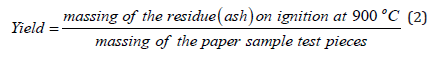
Determination of residue (ash) on ignition at 900 °C
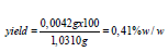
The residue on ignition was the mass of the residue left after incineration of each of the two samples of soft paper in the furnace at 900 °C. The samples of soft paper were weighed in the porcelain heat-resistant dish and were incinerated at 900 °C in the muffle furnace. The masses of the residues were determined by weighing the dishes after incineration of the soft paper samples. The procedure was carried out in duplicate for each of the two soft paper samples. The yield was 0.41%w/w for soft paper roll 1. The yield was 0.37%w/w for the soft paper roll 2. The yield was calculated as the following formula:
For the determination of the ash content, the test pieces of 50g
total weight were prepared, that were cut from different points of
each of the two soft paper sample rolls and were kept into the two
separate glass containers. The paper test specimens consisted of a
number of small pieces having dimensions of 10mmx10mm, and
of size 1cm2. The test pieces of the two paper samples and their
weighing containers were put into the drying oven Memmert GmbH
UNE 400, for 24 hours approximately with a temperature of 105
°C±2 °C. Then the paper small pieces were allowed to attain room
temperature in the desiccator for 40min.
Firstly, for the determination of the ash content of the two paper
samples the button of the muffle furnace Carbolite was pressed to
being operative in place I. The button to adjust the temperature was
then on and the furnace made a short, test cycle. The light of heating
of the furnace was on and was blinking as the furnace reached the
temperature that was put at 900 °C±25 °C, namely 918 °C. The
procedure of calculating the ash content in the two paper samples
was carried out in duplicate. The ash content was weighed 0,0042g
for the soft paper sample 1. The ash content was also weighed
0,0040g for the soft paper sample 2. The portions to be incinerated
consisted of a number of small paper test pieces and had a total
mass of 1,0310g, for the soft paper sample 1
 (3), and 1,0717g for the soft paper sample
2
(3), and 1,0717g for the soft paper sample
2
i.e 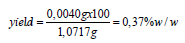 (4) according to equation (2). The
weighing of the samples was performed on the electronic balance
Sartorius Basicplus.
(4) according to equation (2). The
weighing of the samples was performed on the electronic balance
Sartorius Basicplus.
The dishes with the samples were heated first in the Bunsen burner slowly in a manner that the sample burned but did not burst into flames, until the residue in the dish did not release fumes (soot). When the combustion was complete, so that only the small amounts of carbon were visible, the dish was exposed to full heat (900 °C±25 °C) in the muffle furnace for 1hour. When the heating was complete the operation of the furnace was stopped, and we have waited until the temperature in its interior reached 400 °C. Then the dishes with the ash were removed from the furnace and were allowed to attain room temperature in the desiccator for 3 hours. The dishes with the ash content were weighed in the electronic balance with an accuracy of 0.1mg. The furnace was placed in a hood and was provided with a chimney for evacuating the smoke and fumes.
Result and Discussion
Tensile properties (Figure 1-4), The tensile strength was the maximum stress until the fiber network of the paper samples broke, and it was dependent on the degree of fiber-fiber bonding. The inter fiber bonding was the most important factor contributing to the tensile strength property [16]. The soft paper samples were as usual stronger in the Machine Direction (MD) than Counter Machine Direction (CD) direction in tension. The soft papers manufactured on a paper machine, had more fibers oriented in the machine direction than in the cross direction. In general papers have different properties in the machine and the cross direction. The tensile strengths were the maximum stress until the paper fiber network broke. This paper property was dependent on the degree of fiber-fiber bonding. Usually, the soft paper is stronger in MD (Machine Direction) than CD (Cross Direction) in tension. Of all the properties that explained the tensile strength of the cellulose material i.e., the chemical pulp by far the most important was the intermolecular bonding forces. The second soft paper sample tested had a higher tensile strength than the first because of the effect of its extended hydrogen bonding. The -OH and -O-groups in cellulose provided sites for hydrogen bonding governing the tensile properties of the paper samples [19]. The nature of the inter fiber bonds in the soft paper samples were the same as that of the intermolecular bonds in cellulose. The tensile properties in this work were carried out according to ISO 12625-4 [20] and ISO 12625-5 [21]. Ten specimens were tested lengthwise (MD) and ten specimens were tested crosswise (CD) and the median value was taken for each dimension [22]. The soft paper sample 1 had the tensile index [1] 6.67KN.m/Kg lengthwise (MD) and 2.68KN.m/Kg crosswise (CD). The soft paper sample 2 had the tensile index [1] 6.82KN.m/Kg lengthwise (MD) and 2.79KN.m/Kg crosswise (CD). The elongation at rupture [23] of the dry soft paper sample 1 was 14.0% lengthwise (MD) and 9.3% crosswise (CD). The elongation at rupture of the dry soft paper sample 2 was 13.3% lengthwise (MD) and 8.2% crosswise (CD). The elongation at rupture [23-28] of the wet soft paper sample 1 was 8.2% lengthwise (MD) and 7.1% crosswise (CD). The elongation at rupture of the wet soft paper sample 2 was 6.3% lengthwise (MD) and 5.4% crosswise (CD).
Figure 1: Tensile force of the dry soft paper sample 1 as a function of the strain of its paper specimens .

Figure 2:Tensile force of the wet soft paper sample 1 as a function of strain of its paper specimens.

Figure 3:Tensile force of the dry soft paper sample 2 as a function of strain of its paper specimens .

Figure 4:Tensile force of the wet soft paper sample 2 as a function of strain of its paper specimens.

In Table 1 the tensile strengths for the two soft paper samples in
the dry conditioned state are presented as well as their uncertainties
which were calculated as the following formula: (5), where ȳ the mean value of the ten measurements and s is the
standard deviation and n the number of tests made. The theoretical
is from tables for student’s t-distribution for 95% confidence level
and n-1 degrees of freedom, of two ends. In Table 2 the tensile
strengths for the two soft paper samples in dry conditioned state
are presented as well as their uncertainties which were calculated
as the following formula :
(5), where ȳ the mean value of the ten measurements and s is the
standard deviation and n the number of tests made. The theoretical
is from tables for student’s t-distribution for 95% confidence level
and n-1 degrees of freedom, of two ends. In Table 2 the tensile
strengths for the two soft paper samples in dry conditioned state
are presented as well as their uncertainties which were calculated
as the following formula : (6), where ȳ the mean
value of the ten measurements, and s is the standard deviation
and n the number of tests made. The theoretical is from tables for
student’s t-distribution for 95% confidence level and n-1 degrees
of freedom, of two ends. In Table 3 the tensile strengths for the two
soft paper samples in wet conditioned state are presented as well as their uncertainties which were calculated as the following formula
:
(6), where ȳ the mean
value of the ten measurements, and s is the standard deviation
and n the number of tests made. The theoretical is from tables for
student’s t-distribution for 95% confidence level and n-1 degrees
of freedom, of two ends. In Table 3 the tensile strengths for the two
soft paper samples in wet conditioned state are presented as well as their uncertainties which were calculated as the following formula
:  (7), where ȳ the mean value of the ten
measurements, and s is the standard deviation and n the number of
tests made. The theoretical is from tables for student’s t-distribution
for 95% confidence level and n-1 degrees of freedom, of two ends.
In Table 4 the tensile strengths for the two soft paper samples in
wet conditioned state are presented as well as their uncertainties
which were calculated as the following formula :
(7), where ȳ the mean value of the ten
measurements, and s is the standard deviation and n the number of
tests made. The theoretical is from tables for student’s t-distribution
for 95% confidence level and n-1 degrees of freedom, of two ends.
In Table 4 the tensile strengths for the two soft paper samples in
wet conditioned state are presented as well as their uncertainties
which were calculated as the following formula :  (8) where ȳ the mean value of the ten measurements and s is the
standard deviation and n the number of tests made. The ttheoretical
is from tables for student’s t-distribution for 95% confidence
level and n-1 degrees of freedom, of two ends. In Table 5 various
properties for the two soft paper samples are presented as well as
their ash on ignition content and their extended uncertainties at
95% confidence level.
(8) where ȳ the mean value of the ten measurements and s is the
standard deviation and n the number of tests made. The ttheoretical
is from tables for student’s t-distribution for 95% confidence
level and n-1 degrees of freedom, of two ends. In Table 5 various
properties for the two soft paper samples are presented as well as
their ash on ignition content and their extended uncertainties at
95% confidence level.
Table 1: The tensile strengths for the two soft paper samples in the dry conditioned state are presented as well as their
uncertainties which were calculated as the following formula:  (5), where ȳ the mean value of the
ten measurements and s is the standard deviation and n the number of tests made. The theoretical is from tables for
student’s t-distribution for 95% confidence level and n-1 degrees of freedom, of two ends.
(5), where ȳ the mean value of the
ten measurements and s is the standard deviation and n the number of tests made. The theoretical is from tables for
student’s t-distribution for 95% confidence level and n-1 degrees of freedom, of two ends.

Table 2: The tensile strengths for the two soft paper samples in dry conditioned state are presented as well as their
uncertainties which were calculated as the following formula :  (6), where ȳ the mean value of the
ten measurements, and s is the standard deviation and n the number of tests made. The theoretical is from tables for
student’s t-distribution for 95% confidence level and n-1 degrees of freedom, of two ends.
(6), where ȳ the mean value of the
ten measurements, and s is the standard deviation and n the number of tests made. The theoretical is from tables for
student’s t-distribution for 95% confidence level and n-1 degrees of freedom, of two ends.

Table 3: The tensile strengths for the two soft paper samples in wet conditioned state are presented as well as their
uncertainties which were calculated as the following formula  (7), where ȳ the mean value
of the ten measurements, and s is the standard deviation and n the number of tests made. The ttheoretical is from tables for
student’s t-distribution for 95% confidence level and n-1 degrees of freedom, of two ends.
(7), where ȳ the mean value
of the ten measurements, and s is the standard deviation and n the number of tests made. The ttheoretical is from tables for
student’s t-distribution for 95% confidence level and n-1 degrees of freedom, of two ends.

Table 4:The tensile strengths for the two soft paper samples in wet conditioned state are presented as well as their
uncertainties which were calculated as the following formula :  (8) where ȳ the mean value of the ten
measurements and s is the standard deviation and n the number of tests made. The ttheoretical is from tables for student’s
t-distribution for 95% confidence level and n-1 degrees of freedom, of two ends.
(8) where ȳ the mean value of the ten
measurements and s is the standard deviation and n the number of tests made. The ttheoretical is from tables for student’s
t-distribution for 95% confidence level and n-1 degrees of freedom, of two ends.

Table 5: Substrate details.

Calculation of Kubelka-Munk K/S values for the soft paper
sample 1 and for the soft paper sample 2 (absorption coefficient/
scattering coefficient ratio). The optical properties of the soft paper
samples were examined using a UV-visible Spectrophotometer [29]
at room temperature [30]. The K/S ratio for the soft paper sample 1
was found K/S=43.16 and the reflectance ISO brightness used was
measured 88.30%.The ISO brightness measured was the numerical
value of the reflectance of the soft paper sample 1 at 457nm, blue
light reflectance.
The K/S ratio for the second soft paper sample 2 was found
K/S=43.17 and the reflectance ISO brightness used was measured
88.32%. The ISO brightness measured was the numerical value
of the reflectance of the soft paper sample 2 at 457nm, blue light
reflectance.
In this work the Kubelka-Munk theory was used for predicting
the optical properties for the two soft paper samples. The
appearance of the soft papers in the rolls was the result of their
optical properties. As known the Kubelka-Munk theory is based on
the assumption that the interaction between the diffuse light and
the paper material can be described in terms of two fundamental
optical constants. The specific scattering coefficient (S) and the
specific absorption coefficient (K). The Kubelka-Munk theory holds
strictly for homogeneous materials only, and it works well here for
the two paper samples containing chemical pulp [30]. The equation
of Kubelka-Munk used above is: K/S=(1-R͚)2/2R͚ (9) where K is the
absorption or coefficient of reflectivity and S is the coefficient of
light scattering; R͚ is the observed reflectivity for monochromatic
light.
Estimation of the band gap energy Eg from the DRS studies of the soft paper sample 1
A graph was plotted of (k/s hv)2 versus hv . The extrapolation of straight line to (k/s hv)2=0(10) axis (Tauc Plot) gave the value of the band gap energy (Eg)[31]. The estimation of the band gap energy was performed from the DRS (Diffuse reflectance spectra) study. The band gap energy (Eg) [32,33] of the chromophores, i.e., colored compounds, present in the cellulose matrix [34] was estimated as 1.169845eV for permitted indirect transitions, or 1.874091193540620E-19Joules, for the soft paper sample 1. The band gap energy was calculated from the function trend in the excel spreadsheet with the data calculated for the whole range of wavelengths 400-700nm [35,36]; (Figure 5 & 6). The band gap energy (Eg) [33] of the chromophores, i.e., colored compounds, present in the cellulose matrix [34] of the soft paper sample 2 was estimated as 1.169845eV for the permitted indirect transitions, or 1.874091193540630E-19Joules.
Figure 5:(k/s hv)2 versus hv graph of the cellulosic chromophores i.e C=O group [37] and ethylenic double bonds, in the soft paper sample 1 consisting of 100% cellulose, for the calculation of band gap energy for permitted indirect transitions n=2

Figure 6:(k/s hv)2 versus hv graph of the cellulosic chromophores i.e C=O group [37] and ethylenic double bonds, in the soft paper sample 2 consisting of 100% cellulose, for the calculation of band gap energy for permitted indirect transitions n=2.

Application in the mechanics of the system of the Runge-Kutta method [37-39] for finding the position and velocity of the body bound in the wet strip of the two soft roll paper samples. Suppose we have accepted that the body of mass m=2N was attached to the spring constrained to oscillate along the x-axis i.e. horizontally, here the wet soft paper sample strip of dimensions 90x50mm, and with constant k=(4.50/2)=2.25N/m lengthwise, which was the tensile force of the wet tissue paper sample 1, then this body may have felt not only the spring’s force but also the damping force proportional to the square of its velocity and with a ratio of proportion four (4). The weight force of the body was ignored in the supposition. Also, for the wet soft paper sample 2 the constant was k=(4.84/2)=2.42N/m lengthwise. When this body was prevented from the equilibrium position to the position x=2m and was released at the time t=0 then its position and its velocity at the time t=5s could have been calculated with the fourth order improved Runge-Kutta method with pace h=0.5s. Then the graphical representation of its position and velocity for 0<t<5s had to be drawn. Because the damping power of the spring was proportional to the square of the velocity of the body then from the fundamental law of dynamics, we wrote the equations below
mx’’=FE-b|x'|x’ (11), where m was the mass of the body tied to the wet paper sample strip 1, FE was the spring’s force and -b|x'|x’ was the damping force. Then replacing with numbers, we had
2x’’=-4.50x-4|x'|x’(12) for wet tissue paper strip 1 or
x’’=-2.25x-2|x'|x’ (13) for wet tissue paper strip 1, and analogously
2x’’=-4.84x-4|x'|x’ (14) for wet tissue paper strip 2 or
x’’=-2.42x-2|x'|x’ (15) for wet tissue paper strip 2.
Then we set y=x’ and the above equations became
y’=-2.25x-2y|y| (16) for wet tissue paper strip 1 and
y’=-2.42x-2y|y| (17) for wet tissue paper strip 2.
For the solution of the above system, we applied the method of Runge-Kutta fourth class with
f(t, x, y)=y (18)
And for each wet soft paper strip we had the equations
g(t,x,y)=-2.25x-2y|y| (19)and pace h=0.5 in Matlab program for wet soft paper strip 1 and
g(t,x,y)=-2.42x-2y|y| (20) and pace h=0.5 in Matlab program for wet soft paper strip 2
Application in the mechanics of the system of the Runge-Kutta method for finding the position x and the velocity y of the body bound in the wet strip of soft roll paper sample 1 with pace h=0.5s. From the execution in MATLAB program, the solution for the wet soft paper strip 1 of Figure 7a resulted. The solution also for the position x and the velocity y of the body at the time t=5s for paper sample strip 1 was:
x(5)=0.1496m=14.96cm and
u(5)=y(5)=0.0791m/s
Figure 7a: The blue line is the position x in m of the wet paper sample strip 1, and u in m/s the red line is the velocity of the wet paper sample 1 with pace h=0.5s.

Figure 7b: The blue line is the position x in m of the wet paper sample strip 1, and u in m/s the red line is the velocity of the wet paper sample 1, and the grey line is the energy E in Joules for the wet paper sample strip 1, where K=2.25N/m was the spring’s force, with time interval t=0.25s, and pace h=0.5s.

Also, the graph with the solution of Figure 7b resulted where the Energy in Joules for the wet paper strip 1 is also presented. The graph with the grey line for the Energy in Joules of the system was constructed for all the solutions for the position and the velocity of the body for time 0s to 5s. The code in MATLAB for the solving of the system for wet paper sample 1 with the method Runge-Kutta fourth class is presented in Figure 8. The solution of the code in MATLAB for the solving of the system for wet paper sample 1 with the method Runge-Kutta fourth class is also presented with pace h=0.5s in Figure 9. Application in the mechanics of the system of the Runge-Kutta method for finding the position and the velocity of the body bound in the wet strip of the soft roll paper sample 2 with pace h=0.5s. From the execution in MATLAB program the solution for the wet soft paper strip 2 of Figure 10a resulted.
Figure 8:The code in matlab for the solving of the system for wet paper sample 1 with the method Runge- Kutta fourth class is presented above.

Figure 9:The solution of the code in matlab for the solving of the system for wet paper sample 1 with the method Runge-Kutta fourth class is also presented above with pace h=0.5s.

Figure 10a:The blue line is the position x in m of the wet paper sample strip 2 and u in m/s, the red line, is the velocity of the wet paper sample 2 with pace h=0.5s

Figure 10b:The blue line is the position x in m of the wet paper sample strip 2 and u in m/s, the red line, is the velocity of the wet paper sample 2, and the grey line is the energy E in Joules for the wet paper sample 2 where K=2.42N/m was the spring’s force, with time interval t=0.25s, and pace h=0.5s.

Also the graph with the solution of Figure 10b resulted where
the energy in Joules for the wet paper strip 2 was also presented.
The graph for the energy with the grey line was constructed for all
the solutions for the position and the velocity of the body from time
0s to 5s. The code in MATLAB for the solving of the system for wet
paper sample 2 with the method Runge-Kutta fourth class was as in
Figure 11. The solution of the code in MATLAB for the solving of the
system for wet paper sample 2 with the method Runge-Kutta fourth
class is also presented in Figure 12.
From the execution the solution of Figure 10a resulted, as well
as and that for the position and the velocity of the body at the time
t=5s which were for paper sample strip 2
x(5)=0.1585m=15.85cm and
u(5)=y(5)=0.0147m/s
Figure 11:The code in matlab for the solving of the system for wet paper sample 2 with the method Runge- Kutta fourth class and pace h=0.5s is presented above.

Figure 12:The solution of the code in matlab for the solving of the system for wet paper sample 1 with the method Runge-Kutta fourth class is also presented above.

Application in the mechanics of the system of the Runge-Kutta method for finding the position and velocity of the body bound in the wet strip of the soft roll paper sample 1 with pace 0.25s. From the execution in MATLAB program the solution for the wet soft paper strip 1 with pace h 0.25s of Figure 13a resulted. Also, the graph with the solution of Figure 13b resulted where the energy in Joules for the wet paper strip 1 was also presented. The graph for the energy with the grey line was constructed for all the solutions for the position and the velocity of the body from time 0s to 5s.
For the solution of this system, we have applied the method of Runge-Kutta fourth class with pace h=0.25s
f(t, x, y)=y (18)
g(t,x,y)=-2,25x-2y|y| (19)and with pace h=0.25s in the Matlab program
g(t,x,y)=-2,42x-2y|y| (20) and with pace h=0.25s in the Matlab program
Then the graphical representation of its position and velocity for 0<t<5s was drawn.
From the execution the solution of Figure 13a resulted, as well as and that for the position and the velocity of the body at the time t=5s which were for paper sample strip 1
x(5)=0.1927m=19.27cm and
u(5)=y(5)=0.0548m/s
Figure 13a:The blue line x in m is the position of the wet paper sample strip 1 and u in m/s the red line is the velocity of the wet paper sample 1 with pace h=0.25s.

Figure 13b:The blue line is the position x in m of the wet paper sample strip 1, and u in m/s the red line is the velocity of the wet paper sample 1, and the grey line is the energy E in Joules for the wet paper sample strip 1, where K=2.25N/m is the spring’s force, with time interval t=0.25s, and pace h=0.25s.

Figure 14:The code in matlab for the solving of the system for wet paper sample 1 with the method Runge- Kutta fourth class and with pace h=0.25s is presented above.

The code in MATLAB for the solving of the system for wet paper
sample 1 with the method Runge-Kutta fourth class and with pace
h=0.25s was as presented in Figure 14.
The solution of the code in MATLAB for the solving of the system
for wet paper sample 1 with the method Runge-Kutta fourth class
with pace h=0.25s is also presented in Figure 15.
Figure 15:The solution of the code in matlab for the solving of the system for wet paper sample 1 with the method Runge-Kutta fourth class with pace h=0.25s is also presented above.

Application in the mechanics of the system of the Runge-Kutta
method for finding the position and velocity of the body bound in
the wet strip of the soft roll paper sample 2 with pace h=0.25s.
From the execution in MATLAB program the solution for the wet
soft paper strip 2 of Figure 16a resulted. Also, the graph with the
solution of Figure 16b resulted where the energy in Joules for the
wet paper strip 2 was also presented. The graph for the energy with
the grey line was constructed for all the solutions for the position
and the velocity of the body from time 0s to 5s.
g(t,x,y)=-2.42x-2y|y| (20) and with pace h=0.25 in Matlab
program
Figure 16a:The blue line is the position x in m of the wet paper sample strip 2 and the red line is the velocity u in m/s of the wet paper sample 2 with pace h=0.25s.

Figure 16b:The blue line is the position x in m of the wet paper sample strip 2 and u in m/s, the red line, is the velocity of the wet paper sample 2, and the grey line is the energy E in Joules for the wet paper sample 2 where K=2.42N/m is the spring’s force, with time interval t=0.25s, and pace h=0.25.

From the execution the solution of Figure 16a resulted, as well
as and that for the position and the velocity of the body at the time
t=5s which are for paper sample strip 2
x(5)=0.2008m=20.08cm and
u(5)=y(5)=-0.0284m/s
The code in MATLAB for the solving of the system for wet
paper sample 2 with the method Runge-Kutta fourth class was as
presented in Figure 17. The solution of the code in MATLAB for the
solving of the system for the wet paper sample 2 with the method
Runge-Kutta fourth class with pace h=0.25s is also presented in
Figure 18.
Figure 17:The code in matlab for the solving of the system for wet paper sample 2 with pace h=0.25s with the method Runge-Kutta fourth class is presented above.

Figure 18: The solution of the code in matlab for the solving of the system for the wet paper sample 2 with the method Runge-Kutta fourth class with pace h=0.25s is also presented above.

Finally, the benefit of having the above two approximations to the results was the extrapolation calculated below which was used to obtain the best estimate of the solutions we had obtained for the position of the body attached to the wet soft paper strips. Since the Runge-Kutta method was accurate through h4, the two solutions were combined to eliminate the first term of the error (~h5)[38,39] and x(h) and x(h/2) were the two solutions for the position of the body at the time t=5s, with paces h=0.5s and h/2=0.25s respectively. The extrapolated values were found as the formula:
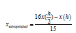 (21), where h was the size of the step. To verify the
accuracy of the method we used Richardson’s extrapolation [40]
and we obtained the below approximations and a better estimate of
the respective derivatives. For the soft paper sample 1 the position
of the body xextrapolated was then found
(21), where h was the size of the step. To verify the
accuracy of the method we used Richardson’s extrapolation [40]
and we obtained the below approximations and a better estimate of
the respective derivatives. For the soft paper sample 1 the position
of the body xextrapolated was then found  (22).
For the soft paper sample 2 the position of the body xextrapolated was
then found
(22).
For the soft paper sample 2 the position of the body xextrapolated was
then found  [23].
[23].
Conclusion
In this work we used an optical microscope to examine the cellulose contents of two soft paper samples which were identified as chemical pulps using the Herzberg staining test. The role of cellulose was to impart the mechanical properties of the two papers which were tested with a tensile-strength machine of 50N. The micro-tensile system used was well suited for measuring the mechanical properties of thin paper samples with large strain (>5%). Then we calculated above the solution of the system of the two wet paper sample strips with a body attached to them, an oscillating horizontally problem, involving two ordinary differential equations (16) and (17), and with two different step sizes h and h/2. We have compared the results for the velocity of the body tied to the two wet soft paper strips made from cellulose which were tested for their tensile strength. The easiest way to accomplish the comparison of the accuracy of that solution was to use the step sizes h and h/2. As a check on the accuracy, the calculations were repeated for the two different step sizes and the results were compared. We also have calculated the Richardson’s extrapolated values of the derivatives.
References
- Lopez F, Perez A, Garcia JC, Feria MJ, Garcia MM, et al. (2011) Cellulosic pulp from Leucaena diversifolia by soda-ethanol pulping process. Chemical Engineering Journal 166(1): 22-29.
- ISO 9184-1:1990, Paper, board and pulps-Fibre furnish analysis Part 1: General Method.
- ISO 9184-2:1990 (1990) Paper, board and pulps-Fibre furnish analysis Part 2: Staining Guide.
- ISO 9184-2:1990 (1990) Paper, board and pulps-Fibre furnish analysis Part 3: Herzberg staining test.
- Mejia LPA, Orea AC, Monsalvo VMA, Sanchez AL, Azuara AH, et al. (2020) Evaluation of tensile force in a porcine trachea using a reflective optical method. Journal of Spectroscopy, p. 6.
- Liu R, Wang H, Li X, Ding G, Yang C (2008) A micro-tensile method for measuring mechanical properties of MEMS materials. Journal of Micromechanics and Microengineering 18(6).
- Li J, Jia Y, Li T, Zhu Z, Zhou H, et al. (2020) Tensile behavior of acrylonitrile butadiene styrene at different temperatures. Advances in Polymer Technology, p. 10.
- Hassan RRA, Ali MF, Fahmy AGA, Ali HM, Salem MZM (2020) Documentation and evaluation of an ancient paper manuscript with leather binding using spectrometric methods. Journal of Chemistry, p. 10.
- Nahar S, Hasan M (2012) Effect of chemical composition, anatomy and cell wall structure on tensile properties of bamboo fiber. Engineering Journal 17(1): 61-68.
- Whitney SEC, Gothard MGE, Mitchell JT, Gidley MJ (1999) Roles of cellulose and xyloglucan in determining the mechanical properties of primary plant cell walls. Plant Physiology 121: 657-663.
- Wei J, Rao F, Huang Y, Zhang Y, Qi Y, et al. (2019) Structure, mechanical performance, and dimensional stability of radiata pine (Pinus radiate D.Don) Scrimbers. Advances in Polymer Technology, p. 8.
- Cheng D, Zhang X, Wang S, Liu L (2019) Effect on mechanical and thermal properties of random copolymer polypropylene/microcrystalline cellulose composites using T-ZnOw as an additive. Advances in Polymer Technology, p. 16.
- Hussain KA, Ismail F, Senu N, Rabiei F (2017) Fourth order improved runge-kutta method for directly solving special Third-order ordinary differential equations. Iranian Journal of Science and Technology Transactions A: Science 41(2): 429-437.
- ISO 287:2017 (2017) Paper and board-Determination of moisture content of a lot-Oven drying method.
- ISO 187:1990 (1990) Paper, board and pulps-Standard atmosphere for conditioning and testing and procedure for monitoring the atmosphere and conditioning of samples, p. 12.
- Lavoine N, Desloges I, Khelifi B, Bras J (2014) Impact of different coating processes of microfibrillated cellulose on the mechanical and barrier properties of paper. Journal of Materials Science 49: 2879-2893.
- Taylor l, Phipps J, Blackburn S, Greenwood R, Skuse D (2020) Using fibre property measurements to predict the tensile index of microfibrillated cellulose nanopaper. Cellulose 27: 6149-6162.
- Liu K, Sun Y, Zhou R, Zhu H, Wang J, et al. (2009) Carbon nanotube yarns with high tensile strength made by a twisting and shrinking method, Nanotechnology 21(4): 7.
- Wang L, Fu W, Peng W, Xiao H, Li S, et al. (2019) Enhancing mechanical and thermal properties of polyurethane rubber reinforced with polyethylene glycol-g-graphene oxide. Advances in Polymer Technology, p. 11.
- ISO (International Standard) 12625-4: 2005 Tissue paper and tissue products-Part 4: Determination of tensile strength, stretch at break and tensile energy absorption.
- ISO (International Standard) 12625-5: 2005 Tissue paper and tissue products-Part 5: Determination of wet tensile strength.
- Mousa A, Heinrich G, Kretzschmar B, Wagenknecht U, Das A (2012) Utilization of agrowaste polymers in PVC/NBR alloys: Tensile, thermal, and morphological properties. International Journal of Chemical Engineering, p. 5.
- Niazmand R, Razavizadeh BM, Sabbagh F (2020) Low-density polyethylene films carrying ferula asafoetida extract for active food packaging: Thermal, mechanical, optical, barrier, and antifungal properties. Advances in Polymer Technology, p. 15.
- ISO DIS 2470-1:2008 Paper, board and pulps-Measurement of diffuse blue reflectance factor-part 1: Indoor daylight conditions (ISO brightness).
- ISO 2471:2008 (2008) Paper and board-Determination of opacity (paper backing)-Diffuse reflectance method.
- ISO (International Standard) 2144:2019: Paper, board, pulps and cellulose nanomaterials-Determination of residue (ash content) on ignition at 900 °C.
- ISO 536:1995 Paper and board-Determination of grammage.
- Tappi T432 om-87: Water absorbency of bibulous papers.
- Yang AP, Ma MH, Li XH, Xue MY (2012) Interaction of irbesartan with bovine hemoglobin using spectroscopic techniques and molecular docking. Spectroscopy: An International Journal 27(2): 119-128.
- Siddiqui SA, Rasheed T, Faisal M, Pandey AK, Khan SB (2012) Electronic structure, nonlinear optical properties and vibrational analysis of gemifloxacin by density functional theory. Spectroscopy: An International Journal 27(3): 185-206.
- Malcic VD, Mikocevic ZB, Itric K (2012) Kubelka-munk theory in describing optical properties of paper (II) tehnicki vjesnik 19(1): 191-196.
- Parhi P, Manivannan V, Kohli S, McCurdy P (2008) Synthesis and characterization of M3V2O8 (M=Ca, Sr and Ba) by a solid-state metathesis approach. Bull Mater Sci 31(6): 885-890.
- Li P, Abe H, Ye J (2014) Band-gap engineering of NaNbO3 for photocatalytic H2 evolution with visible light. Int J Photoenergy, pp. 1-6.
- Hettegger H, Amer H, Zwirchmayr NS, Bacher M, Hosoya T, et al. (2019) Pitfalls in the chemistry of cellulosic key chromophores. Cellulose 26: 185-204.
- Morales AE, Lopez IIR, Peralta MDR, Carrillo LT, Cantu MS, et al. (2019) Automated method for the determination of the band gap energy of pure and mixed powder samples using diffuse reflectance spectroscopy. Heliyon 5(4): 1-19.
- Abdullahi SS, Guner S, Koseoglu Y, Musa IM, Adamu BI, et al. (2016) Simple method for the determination of band gap of nanopowdered sample using kubelka munk theory. J Nig Assoc of Mathem Physics 35: 241-246.
- Casanova EGO, Mandujano HAT, Aguirre MR (2019) Microscopy and spectroscopy characterization of carbon nanotubes grown at different temperatures using cyclohexanol as carbon source. Journal of Spectroscopy, p. 6.
- England R (1969) Error estimates for Runge-Kutta type solutions to systems of ordinary differential equations. The Computer Journal 12(2): 166-170.
- Chai AS (1968) Error estimate of a fourth-order Runge-Kutta method with only one initial derivative evaluation. IEEE Computer Science 1: 467-471.
- DeVries PL (1994) A First Course in Computational Physics. John Wiley & Sons, Inc., USA.
© 2021 Chryssou K. This is an open access article distributed under the terms of the Creative Commons Attribution License , which permits unrestricted use, distribution, and build upon your work non-commercially.
Editor In Chief


.jpg)


Signup for Newsletter

Quick Links
 Editorial Board Registrations
 Submit your Article
 Refer a Friend
 Advertise With Us
Our Recent Edition

.jpg)


Top Editors


.jpg)


.bmp)
.jpg)
.png)
.jpg)


.jpg)


.png)

.png)


.png)


Financial Support

Sponsors

Latest e-Books

Latest Video

 a Creative Commons Attribution 4.0 International License. Based on a work at www.crimsonpublishers.com.
Best viewed in
a Creative Commons Attribution 4.0 International License. Based on a work at www.crimsonpublishers.com.
Best viewed in