How to Select X-axis Values when the Independent Variable Spans Several Orders of Magnitude

When designing experiments, researchers often need to measure a dependent variable, such as the response of an instrument or method, with respect to an independent variable such as the concentration of a reactant. Often the independent variable spans several orders of magnitude, (e.g., when experimental concentrations range from 0.0100mM to 10.0mM), which can make it difficult to construct a clear graph of the data. In such situations, it is more appropriate to plot the independent variable on a logarithmic axis (usually the base 10 logarithmic scale) rather than a linear axis, in order to avoid superimposed data points and to make the graph easier to interpret. By convention, the independent variable is usually plotted horizontally as the x-axis or abscissa, and the dependent variable is plotted vertically as the y-axis or ordinate.

After choosing the range of values to be measured for the independent variable to accommodate experimental goals, researchers then decide the number of data points to collect (the sample size) within the chosen range, so that a statistically reliable measurement can be performed and a valid conclusion can be drawn from the data. The determination of sample size is addressed by other sources [1,2] and useful websites allow users to make actual sample size calculations (e.g., http://www.biomath.info/power/index.html and http://davidmlane.com/hyperstat/power.html).

Once the sample size has been chosen, the next step is to determine the points within the independent variable’s range where experimental measurements will be taken. For example, to determine the binding constant of a divalent ion to a protein, if 12 different concentrations of the ionic solution ranging from 0.0100mM to 10.0mM are to be prepared in order to obtain their fluorescence at a given wavelength, which 12 concentrations will allow the values to be equally spaced on a logarithmic axis? To answer this question, the author introduces a straightforward approach for calculating these values.

To continue with the above example, we must select 12 concentrations of an independent variable ranging from 0.0100mM to 10.0mM. First, calculate the distance between the largest and smallest values within the range on a logarithmic scale as follows: log[highest value] – log[lowest value]=log10.0 – log0.0100=log(10.0/0.0100)=3.00. Next we must calculate the spacing between our 12 axis values; because there are 11 segments between 12 points, the length of each segment (i.e., the distance between two adjacent values) on a logarithmic scale is calculated by dividing the overall distance by the number of separating segments. For this example, the equation is 3.00/11=0.273.

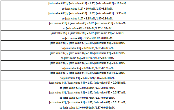
Once the distance between adjacent axis values on the logarithmic scale is known, detailed calculations to determine the value of the measurement can begin from either the highest concentration (i.e., axis value #12) or the lowest concentration (i.e., axis value #1). First, the author illustrates how to work from the highest concentration value; brackets “[ ]” are used to indicate the concentration of the substance at a particular axis value. As calculated above, the distance between axis value #12 and its adjacent axis value #11 on a logarithmic axis is 0.273, meaning that log[axis value #12] – log[axis value #11]=log([axis value #12]/ [axis value #11])=0.273. Thus, the ratio of the concentrations of axis value #12 versus axis value #11 is equal to [axis value #12]/ [axis value #11]=100.273=1.87. Since the concentration of axis value #12 is 10.0mM, the concentration of axis value #11 can be calculated as 10.0mM/1.87=5.35mM. This same approach is then used to calculate the concentrations of the rest of the axis values, as shown in Table 1.

Table 1:Detailed calculations (starting from the highest concentration value) for determining the 12 experimental concentrations to use.

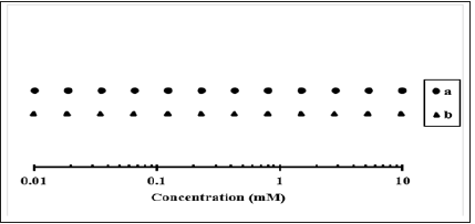
Using the calculated values from Table 1 to set up a graph, Figure 1, line a, shows that the 12 points ranging from 0.0100mM to 10.0mM are equally spaced on a logarithmic axis. If instead, we start the calculations from the lowest concentration value (i.e., axis value #1), we first calculate [axis value #2] / [axis value #1]=100.273=1.87, and since [axis value #1]=0.0100mM, we can determine the concentration of axis value #2, which is [axis value #2]=0.0100mM × 1.87=0.0187mM. Note that when starting with the lowest values on the axis, the concentration is multiplied by the distance factor, rather than divided by it as when starting with the highest values on the axis. Following this pattern, we can then calculate the concentrations of axis values #3#12, which are 0.0350mM, 0.0654mM, 0.122mM, 0.228mM, 0.426mM, 0.797mM, 1.49mM, 2.79mM, 5.22mM, and 9.76mM, respectively. Figure 1, line b, shows that while these values are not quite identical to those in Figure 1, line a, they are equally spaced on the logarithmic axis as well.

Figure 1:Graph plotted using data from Table 1 and the subsequent paragraph. In line a (•), the calculations begin from the highest concentration value; in line b (▲), the calculations begin from the lowest concentration value. Note that both versions result in 12 equally spaced points ranging from 0.0100mM to 10.0mM on a logarithmic axis.

This study provides a detailed, step-by-step guide for determining the points at which experimental measurements will be taken for an independent variable whose range spans several orders of magnitude. Following this method, students and/or researchers should be able to design an appropriate set of experimental measurements and plot their results for optimal clarity.

This work is supported by the National Science Foundation under Award No. OIA-1458952.

All data generated and analyzed during this study are included in this published article.

1. Dell RB, Holleran S, Ramakrishnan R (2002) Sample size determination. ILAR Journal 43(4): 207-213.
2. Charan J, Kantharia ND (2013) How to calculate sample size in animal studies? J Pharmacol Pharmacother 4(4): 303-306.