Effect of Gap between Airfoil and Embedded Rotating Cylinder on the Airfoil Aerodynamic Performance

From the time of Prandtl,1904, the boundary layer concept was introduced and scientists and engineers had been faced a challenge to reduce the adverse effects of boundary layer separation on the performance of various devices such as airfoils, compressor blades, turbine blades, etc. Boundary layer separation takes place under adverse pressure gradient conditions when viscous effects are no longer confined to a thin layer but affect the overall flow pattern drastically. The most common application up to date has been the flow around an airfoil wing of an aircraft. Flow separation takes place on the upper surface of the airfoil at a large angle of attack resulting in a drastic fall in lift. The concept of delaying boundary layer separation has also been used in wing to reduce aerodynamic drag. Invariably this had been done by momentum injection through using rotating cylinder as a concept of moving surface boundary layer with different gap spaces between the airfoil and rotating cylinder and taps on upper and lower surfaces of the airfoils in order to control the flow and improve their lift characteristics.

Modi [1] carried out tests on rotating cylinders located at the leading and trailing edge of the airfoil. The leading edge rotating cylinder extended the lift curve without affecting its slope thus increasing the maximum lift and delaying stall. The trailing edge cylinder acted as a flap and shifted the lift curve to the left thus increasing the lift coefficient before stalling occurs. There are many ways to control of boundary likes using devices to control boundary layer or using very small extended surfaces starting from body that want to control the boundary layer on. Modi [2,3] presented a comprehensive wind-tunnel test program involving a family of airfoils such as NACA 63-218 and Joukowsky with one or more cylinders forming the moving surface. Their results suggested that the leading-edge rotating cylinder increases the maximum lift coefficient and delays the stall angle of attack by (2.73 and 48°), respectively. The study also showed that an increase in (Uc/U∞) to a value greater than 4 does not yield any additional benefit. Also, in different papers, Modi [1] showed that using rotating cylinders results in increasing the maximum lift coefficient by more than 150% and delays the stall angle of attack up to 44°. Adoune [4] presented numerically a study of a flow over a two dimensional symmetric Joukowski airfoil with a rotating cylinder at the leading edge and trailing edge. The result showed an improvement of aerodynamic coefficients with leading edge rotating cylinder, exceeded 240% at an angle of attack 4°, and for the ratio of cylinder velocity to uniform velocity of (Uc/U∞ = 4). While, no effect of trailing edge rotating cylinder on the aerodynamic coefficient was found. Al- Garni et al. [5] showed an experimental investigation conducted on a two- dimensional NACA 0024 airfoil equipped with a leading edge rotating cylinder. The work showed that the leading-edge rotating cylinder increases the lift coefficient of a NACA 0024 airfoil from (0.85 to 1.63) when the cylinder surface velocity ratio increase from (0 to 4). Hussein SH [6] studied the separation control on the NACA 0012 and NACA0018 airfoils by using a rotating cylinder based on the computation of Reynolds-average Navier-Stokes equations. A numerical model based on collocated finite volume method was developed to solve the governing equations on a body- fitted grid. To ensure the accuracy of the code first, second and third order differencing schemes, with and without flux-limiters, had been implemented and tested. The systematical investigation of the rotating cylinder was conducted on the same NACA 0012 airfoil in the range of attack angles from (10°) up and beyond the stall angle at Reynolds number, (Re, =10⁶). The influence of some parameters associated with rotating cylinder, such as its radius, location, and the speed ratio (Uc/U∞) on the performance of the airfoils had been studied. Sahu & Patnaik [7], studied the flow past NACA 0012 airfoil; simulations for different angles of attack varying from (0° to 20°) at Reynolds numbers, (Re=46400). The influence of momentum injection on the fluid flow features, stall angles, lift and drag forces were investigated. Validations were carried out for flow past NACA0012 aerofoil. Simulations were performed for different angles of attack (α) in the sub-critical Reynolds number. It was observed that, stall occurs approximately at (α =120) as the boundary layer separation started at the leading edge for (Re = 46400). They focused on delaying stall angle to achieve the maximum lift force. A simple momentum injection technique was employed with the help of one rotating element-an actuator disc, which was embedded on the leading edge of the aerofoil. The idea was to reduce the relative motion between surface and the fluid flow, and bring high momentum shear layers closer to the no-slip surfaces. The actuator disc was rotated with different angular speeds, for different angles of attack. It was observed that, stall occurred at (α=12°) at (Re=46400). In addition, the stall angle was delayed by using the simple momentum injection technique with the help of one rotating element as an actuator disc on the leading edge of airfoil. At higher angle of attack, the stall angle was significantly delayed due to momentum injection. A delayed stall angle resulted in an attendant to maximum lift coefficient. Due to delay and/or prevention of separation, drag coefficients were also reduced considerably, resulting in a high performance- lifting surface.

Yemenici O [8] investigated experimentally the flow field around NACA 0012 airfoil in a wind tunnel with different Reynolds numbers and angles of attack. The Reynolds number was based on the chord length of airfoil and the attack angle were varied from (97000 to 190000) and (0 to 14) degrees respectively around NACA 0012 airfoil. The pressure coefficient of the suction side of the airfoil initially increased near the leading edge and then showed a monotonously decreased up to trailing edge for all angles of attack. A symmetric pressure distribution was observed along the suction and pressure side of the airfoil at zero attack angles. The angles of stall and lift coefficients increased with Reynolds number. The results showed that the pressure and lift coefficients were displayed a strong dependence on Reynolds number and angles of attack.

The present work investigates the effect of the gap between the airfoil and the rotating cylinder embedded on leading edge of the airfoil on its aerodynamic performance theoretically and experimentally. Symmetrical airfoil four digits, (NACA 0012) with Reynolds number of 700000 will consider in this work. Upon the numerical results of all above considered cases, an optimum configuration of airfoil is found which is represented by gap space between rotating cylinder and leading edge of airfoil for best performance. In addition, the best performance enhancement of unconventional airfoil will predicate.

The starting point of any numerical method is the mathematical model, i.e. the set of partial differential or integral-differential equations and boundary conditions. These equations are based on the conservation of mass and momentum.

Geometry coordinates

The unconventional airfoil under consideration consists of the normal airfoil NACA0012 with embedded leading edge rotating cylinder. The geometry nodes was built up by the developing a computer program to the airfoil equations in the Microsoft Excel program by using the equations of the airfoil boundaries for upper and lower parts and making several modifications to give the exact locations and dimensions of the tap that will be studied.

The geometry of unconventional airfoil is shown in Figure 1, which consists of airfoil with leading edge rotating cylinder. The gap between the rotating cylinder and the airfoil will be varied from (1 to 5]mm. The rotating cylinder diameter is (0.1 c] and chord length, c is (1] m.

Figure 1: Geometry of NACA 0012 airfoil with gap and rotating cylinder.

Assumptions

The following assumptions will be considered.

a. Working fluid is air (7)

b. Steady state flow

c. Two dimensional of mean flow

d. Fully turbulent flow

e. Incompressible flow, (Mach number =0.03]

f. Newtonian fluid

g. No heat transfer and generation

The governing equations

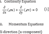
In order to analyze the flow field around the airfoil with rotating cylinder and gap, solution of two-dimensional Navier- Stokes equations is required, due to the complexity of flow around airfoil configurations and the dominancy of viscosity effects. Since the pressure gradient has such a pronounced effect on flow field; therefore, the equations will be represented by pressure gradient along the airfoil, Fox & McDonald [9]. The governing equations for the mean velocity and pressure are the mass and momentum equations, these are analyzed the averaged Navier-Stokes equations. The equations of motion can be written as follows:

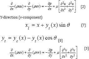
The effects of fluctuation can be introduced by replacing the flow variable u, v, ρ and p by the sum of mean and fluctuating components, Versteeg & Malalasekera [10].

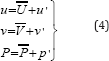
Also, The NACA airfoils are constructed by combining a thickness envelope with a camber or mean line.

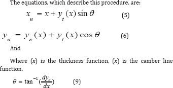
It was unusual to neglect the camber line slope, which simplifies the equations and makes the reverse problem of extracting the thickness envelope and mean line for given airfoil straightforward. The NACA four and five digit series were defined completely by formulas. In both cases, the thickness distribution had given by, Hussein [6]:

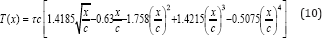
Here (c) is the airfoil chord and (x) is the distance along the chord line from the leading edge. The parameter (τ) is the thickness ratio of the airfoil (maximum thickness/chord). This thickness distribution was derived in 1930 by Eastman, in National Advisory Committee for Aeronautics Langley Laboratory, on the basis of examination of airfoils and known to be an efficient formula.

The NACA 0012 airfoil is symmetrical, the 00 indicating that it has no camber. The 12 indicates that the airfoil has a 12% thickness to chord length ratio: it is 12% as thick as it is long. Figure 2 shows airfoil shape for NACA 4- digit sections.

Figure 2: Parameters used to describe the profile of an airfoil.

Reynolds-averaged navier- stokes equations

The Reynolds-averaged Navier-Stokes equations (RANS equations) are time-averaged equations of motion for fluid flow. The idea behind the equations is Reynolds decomposition, whereby an instantaneous quantity is decomposed into its time-averaged and fluctuating quantities, an idea was first proposed by Osborne Reynolds. The RANS equations are primarily used to describe turbulent flows. These equations can be used with approximations based on knowledge of the properties of flow turbulence to give approximate time-averaged solutions to the Navier-Stokes equations.

The derivation of these equations, details regarding the constitutive relations used and the various turbulence modeling assumptions employed can be found in several references, White [11], Ferziger & Peric [12]. Employing indicial notation, the instantaneous form of continuity and momentum equations in Cartesian coordinates can be written as follows:

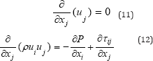
Where (X_i) is position vector, (T_ij) is viscous stress tensor. The constitutive relation between stress and strain rate for a Newtonian fluid is used to relate the components of the stress tensor to velocity gradients:

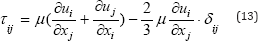
The conservation equations above hold exactly for laminar flows. For turbulent flows, in the context of RANS methods, ensemble averaging will be resorted. The time- averaged form of the above equations for turbulent flows is obtained by mass- averaging. The various flow properties are decomposed into mean and fluctuating components, as follows:

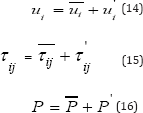
Note that Favre-averaging is used for u_i and T_ij (bar and prime denote a Favre- averaging mean quantity and the fluctuation above this mean, respectively). Reynolds- averaging is used for P (bar and prime denote a Reynolds- Averaged mean quantity and the fluctuation above this mean, respectively).

Computational Fluid Dynamics, commonly known as CFD has becomes an important tool used for the design and analysis of thermal-fluid systems over the last several decades .Increases in computing power have permitted more detailed calculations to be undertaken in significantly less time leading to an expanded envelope for computational modeling. Ultimately, it is desirable to continue the development of newer and more accurate CFD algorithms while benchmarking current computational packages. A detailed summary of the CFD methodology and techniques employed during this study will be discussed in the following sections.

Turbulence models

Turbulence modeling is the construction and using a model to predict the effects of turbulence. Averaging was often used to simplify the solution of the governing equations of turbulence. The K-omega model was a two equations model that means, it includes two extra transport equations to represent the turbulent properties of the flow. The first transported variable is turbulent kinetic energy, K. The second transported variable in this case is the specific dissipation, w.

The Shear-Stress Transport (SST) K-w model: The SST K-w turbulence model is a two-equation eddy-viscosity model developed by Menter [13] to blend effectively the robust and accurate formulation of the K-w model in the near-wall region with the free-stream independence of the K-w model in the far field. The SST K-w model is similar to the standard K-w model, but includes the following refinements:

a. The standard K-w model and the transformed K-w model are both multiplied by a blending function and both models are added together.

b. The blending function is designed to be one in the nearwall region, which activates the standard K-w model, and zero away from the surface, which activates the transformed K-w model.

c. The SST model incorporates a damped cross-diffusion derivative term in the w-equation.

d. The definition of the turbulent viscosity modified to account for the transport of the turbulent shear stress and the modeling constants are different.

These features make the K-w SST model more accurate and reliable for a wider class of flows than the standard K-w model. The K-w SST turbulence model is a combined version of the K-w and K-w turbulence models and governed by:

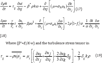
Where Ω is the absolute value of the vorticity, and the function F₂ is given by

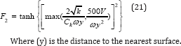
Where (y) is the distance to the nearest surface.

The coefficients β, γ, σk and σ_ωare defined as functions of the coefficients of the K-ω and K-ω turbulence models and they are listed as follows:

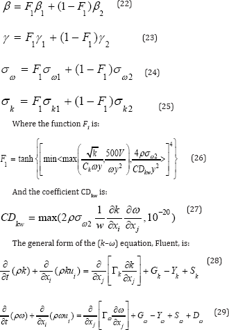
The modeling the effective diffusivity for the k-ω model are given by

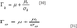
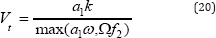
Where σ_k and σ_ωare the turbulent Prandtl numbers for k and ω, respectively. The turbulent viscosity, μ_t is computed by combining k and ω as follows:

Grid generation

In order to solve the governing partial differential equations (PDE) numerically, approximations to the partial differentials are introduced. These approximations convert the partial derivatives to finite volume expression, which are used to rewrite the (PDE) as algebraic equations. The approximate algebraic equations, referred to as finite volume equations, are subsequently solved at discrete points within the domain of interest.

Standard CFD methods require a mesh that fits the boundaries of the computational domain. The generation of computational mesh that is suitable for the discretized solution of twodimensional Navier-Stokes equations has always been the subject of intensive researches. This kind of problem covers a wide range of engineering applications. For a complex geometry, the generation of such a mesh is time consuming and often requires modifications to the model geometry.

Therefore, a set of grid points within the domain, as well as the boundaries of the domain, must be specified. The creation of such a grid system was known as grid generation. In addition, the grid should be arranged so that the nodes are concentrated in areas where the gap affects, Versteeg & Malalasekera [10].

Mesh topology: For unstructured mesh, FLUENT uses unstructured solver which uses internal data structures to assign an order to the cells, faces, and grid points in a mesh and to maintain contact between adjacent cells. This gives the flexibility to use the best grid topology for complex geometry, as the solver does not force an overall structure or topology on the mesh (i.e., it does not require ( i, j, k )indexing to locate neighboring cells). FLUENT code uses different element types for mesh topology. The type of element specifies the number of mesh nodes and the node pattern associated with element shapes.

In the present work, a higher order element type was used for mesh generation to approximate precisely the boundaries of high curvature, as shown in Figure 3 .This included surface mesh, a higher order triangular element with hanging nodes (i.e., nodes on edges that are not vertices of all the cells sharing those edges) was used, as shown in Figure 4.

Figure 3: Mesh near the wall surface of the front rotating cylinder for gap space (3mm) and angle of attack (10°).

Figure 4: Higher order triangular elements surface mesh type.

Figure 5: Mesh independency test for airfoil with rotating cylinder.

Mesh independency test: The way of checking whether the solution is grid independent or not is to create a grid with more cells to compare the solutions of the two models. Grid refinement tests for drag coefficient indicated that a grad size of approximately (100,000 cells) provide sufficient accuracy and resolution to be adopted as the standard for airfoil surface. Figure 5 shows the grid independency test performed for airfoil surface with rotating cylinder.

Experimental tests carried out in a wind tunnel in order to investigate and check the numerical results of flow on the modified NACA 0012 airfoil with rotating cylinder. The experimental works mainly based on selected optimum configuration of airfoil for best performance enhancement of unconventional airfoil from the numerical results. An optimum configuration of airfoil with leading edge embedded rotating cylinder of 50mm diameter and 700mm depth, both airfoil profiles sections are made from wood selected Sahu & Patnaik [7].

The work presents an experimental analysis of such improved performance of airfoil. The experimental investigations were involved the measurements of surfaces pressure distribution and consequentially, calculations of aerodynamic coefficients (lift and drag and their ratio) for normal NACA0012 and unconventional (NACA 0012 with leading edge rotating cylinder) airfoils at a specified Reynolds number (700,000), different angles of attack (0, 5, 10 and 15) degrees, with velocity ratios of rotating cylinder to uniform flow velocity (Uc/U∞=1), with uniform flow velocity of (20m/s).

Numerical results were obtained for flow over a normal (NACA0012) and unconventional airfoil for Reynolds number of (700000), angles of attack (0, 5, 8, 10, 12, and 15) degrees and for velocity ratios of (Uc/U∞= 1, 2, and 3). The results for various gap sizes (1mm to 5mm) were obtained and the optimum case for best airfoil performance was selected.

For experimental work, all above parameters were performed but for velocity ratio of (Uc/U∞=1). The measurements carried out for free stream velocity of (20m/s) and Reynolds number (700000) corresponding to the chord length. Only the measurements were performed at (Uc/U∞=1). This is due to unstable operation of rotating cylinder and fluctuations in pressure distribution measurements for velocity ratios of (2 and 3).

Flow field configurations for various gaps with different velocity ratios (Uc/U∞=1,2 and 3), were studied in the form of lift to drag coefficients ratios to figure out the gap size for best airfoil performance. The flow separation occurs at relatively high angle of attack. The upper surface flow remains attached to the airfoil up to a distance downstream of the leading edge then at it separates and leads to a large separation bubble, with reattached towards the trailing edge. The rotation of the leading edge cylinder resulted in an increase in suction over the nose and the smoothness of the transition from the cylinder to the airfoil surface. The same trend was obtained by Modi, and Mokhtarian, 1988. The results were found for various angles of attack and gaps as shown in Figures 6-8.It can be seen from the Fig. 6, that the maximum lift to drag ratio of (58.936) was obtained for gap (3mm) with velocity ratio of (Uc/ U∞=1 ).

Figure 6: Numerical results of lift to drag coefficients ratio for unconventional airfoil with various angles of attack and gaps space at velocity ratio (Uc/U∞=1) and (Re=700,000).

Figure 7: Numerical results of lift to drag coefficients ratio for unconventional airfoil with various angles of attack and gaps space at velocity ratio (Uc/U∞=1) and (Re=700,000).

Figure 8: Numerical results of lift to drag coefficients ratio of unconventional airfoil with various angles of attack gaps space at velocity ratio (Uc/U∞=3) and (Re=700,000).

Also, lift to drag coefficients ratios of (60.6074 and 62.036] obtained for velocity ratios of (Uc/U∞=2 and 3] respectively, compared with value of (18] for normal airfoil as shown in Figures 6-8. It is clear from figures that, the maximum value of lift to drag coefficients ratios occurred at the same gap for all velocity ratios. This attributed can be claimed to velocity of rotating cylinder besides of the injection of the momentum to the flow stream near the airfoil wall and this will increase the energy of the flow that causes to attach the flow and prevents the separation. At the same time, when the cylinder velocity was increased, the lift to drag coefficients ratio was increased, due to increase in energy of the attached flow. These effects were appeared clearly with increasing the velocity ratio to (Uc/U∞=2 and 3].

Comparison of lift to drag coefficient ratios between experimental and numerical results for unconventional airfoil

Figure 9: Comparison of lift to drag coefficients ratios be-tween numerical and experimental results of unconvention-al airfoil with gap space (1mm).

Figure 10: Comparison of lift to drag coefficients ratios be-tween numerical and experimental results of unconvention-al airfoil with gap space (2mm).

For different gaps (1,2,3,4, and 5mm) and velocity ratio of ( Uc/U∞=1), the lifts to drag coefficients ratios were obtained for unconventional airfoil numerically and experimentally. As shown from Figures 9-13, as the lift coefficient was increased, the corresponding drag coefficient was also decreased for velocity ratio of (Uc/U∞=1] as shown in figures. For numerical results, the maximum value of (54] for lift to drag ratio was obtained at angle of attack (5°] and gap (3mm], while for experimental results a value of (44] for lift to drag ratio was obtained, at angle of attack (5°] and space gap (3mm], with the maximum deviation of (9.5%] [14].

Figure 11: Comparison of lift to drag coefficients ratios be-tween numerical and experimental results of unconvention-al airfoil with gap space (3mm).

Figure 12: Comparison of lift to drag coefficients ratios be-tween numerical and experimental results of unconvention-al airfoil with gap space (4mm).

Figure 13: Comparison of lift to drag coefficients ratios be-tween numerical and experimental results of unconvention-al airfoil with gap space (5mm).

Comparison of experimental and numerical results for normal and unconventional airfoil with previous works

Figure 14: Comparison of lift coefficients of experimental results for normal airfoil (NACA 0012), with Yemenici [8].

The experimental results of lift coefficient, (C_l) for normal airfoil were compared with the experimental results of Yemenici [8] in Figure 14. The figure shows a similar trend for lift coefficients for both results, but the present results have 16% higher values than Yemenici [8]. This difference is due to the different values used for Reynolds number. The (C_l) was increased monotonously with angle attack and reached up the maximum value at the angle attack of (12°) at ( =1.9x105). This result showed the occurrence of the stall at (α = 12°). The maximum (C_l) defined at the stall angle and varied with Reynolds number due to viscous effects.

Figure 15: Comparison of lift coefficients between numer-ical results of the present study at (Uc/U∞ = 1) with Sahu & Patnaik [7].

The numerical results of lift and drag coefficients for unconventional airfoil (NACA 0012) with existence of the gap space (1mm) and rotating cylinder speed ratio (Uc/U∞= 1) were compared with numerical results of Sahu & Patnaik [7] for the same Reynolds numbers in Figure 15 & 16. The present results showed the same trend but with higher values for lift coefficient than the Sahu & Patnaik [7] results. While the results for drag coefficients were showed lower values than Sahu & Patnaik [7] results. These differences may be attributed to numerical dealing of the gap and rotating cylinder. The maximum deviation was (14%).

Figure 16: Comparison of drag coefficients between numer-ical results of the present study at (Uc/U∞=1) with Sahu & Patnaik [7].

On the other hand, comparison of the experimental results of the present work were made for lift and drag coefficient at the (Uc/U∞= 1) of the unconventional airfoil with Sahu & Patnaik [7] as shown in Figure 17 & 18. It was found from figures that the lift coefficient of the present work have higher values than the results of Sahu & Patnaik [7]. While the results for drag coefficients showed lower values than the values of Sahu & Patnaik [7]. These differences were due to various Reynolds numbers used in two results. The maximum deviation was 14% for drag coefficient.

Figure 17: Comparison of experimental results of lift coeffi-cient at (Uc/U∞ = 1) with Sahu & Patnaik [7].

Figure 18: Comparison of experimental results of drag co-efficient at (Uc/U∞ = 1) with Sahu & Patnaik [7].

However, the values of an overall ratio of aerodynamic performance, which represented by ratio of lift to drag coefficient was higher than that reported by Sahu & Patnaik [7].

a The optimum configuration for the unconventional airfoil for numerical results was found to be at velocity ratio of (Uc/U∞= 3] with the space gap (3mm] for best airfoil performance.

b. The maximum lift to drag ratios of (58.9, 60.6 and 62.0] were obtained in numerical results for velocity ratios (Uc/U∞=1, 2 and 3] respectively when compared with value of 18 for normal airfoil.

c. Form numerical results, the maximum values of lift to drag coefficients ratios were occurred at the same gap space (3mm] for all velocity ratios.

d. When the cylinder velocity increased, the lift to drag coefficients ratio increased, These effects were more pronounce with increasing the velocity ratio to (Uc/U∞= 2 and 3].

e. The angle of attack 14 degree was the angle of separation for this airfoil without cylinder at the leading edge of the airfoil, but the separation at this angle was not appeared when the rotating cylinder was used. This due to vortex generation and delaying the separation point.

f. A wide range of pressure drag was observed at high angle of attack for normal airfoil. While, for unconventional airfoil, the drag range was limited and this was due to the gap effect in airfoil with rotating cylinder on airfoil performance.

g. An increase of 35% in lift coefficient for unconventional airfoil with optimum configuration was obtained compared with normal airfoil.

h. A reduction of 21% in drag coefficient for unconventional airfoil with optimum configuration was obtained compared with normal airfoil at the same angle of attack.

1. Modi VJ, Mokhtarian F (1988] Effect of moving surfaces on the airfoil boundary layer control. Aircraft J 27: 42-50.
2. Modi VJ, Sun JLC, Akutsu T, Lake P, McMillan K, et al. (1981] Moving- surface boundary-layer control for aircraft operation at high incidence. Journal of Aircraft 18(11]: 963-968.
3. Modi VJ, Mokhtarian F, Fernando, Yokomizo T (1991] Moving surface boundary-layer control as applied to two-dimensional airfoils. Journal of Aircraft 28(2]: 104-112.
4. Adoune BM (1998] Numerical study of a flow over a two-dimensional airfoil with rotating cylinder at the trailing-edge. M.Sc. Thesis, Mosul University, Iraq.
5. Ahmed, Al-Garni Z, Abdullah, Al-Garni M, Ahmed SA, et al. (2000] Flow control for an airfoil with leading-edge rotation: an experimental study, king fahd university of petroleum and minerals, Dhahran 31261, Saudi Arabia, Journal of Aircraft 37(4].
6. Hussain SH (2005] Numerical investigation of airfoil flow control by means of rotating cylinder, Phd. thesis, mechanical engineering department, University of Baghdad, Iraq.
7. Sahu RD, Patnaik BSV (2010] Momentum injection control of flow past an aerofoil, Proceedings of the 37^th National & 4^th International Conference on Fluid Mechanics and Fluid Power, IIT Madras, Chennai, India.
8. Yemenici O (2013] Experimental investigation of the flow field around NACA0012 airfoil. International Journal of Sciences 2(8]: 98-101.
9. Philip JP, John CL (1973] Fox RW, McDonald AT Introduction to fluid mechanics, (2^nd edn], by John Wiley & Sons, USA.
10. Versteeg HK, Malalasekera W (1995] An introduction to computational fluid dynamics-the finite volume method, Longman group Ltd, UK.
11. White FM (1991] Viscous fluid flow. (2^nd edn], McGraw-Hill, New York, USA.
12. Ferziger JH, Peric M (1999] Computational methods for fluid dynamics. (2^nd edn], Springer, Berlin, Germany
13. Menter FR (1994] Two-equation eddy-viscosity turbulence models for engineering applications. AIAA Journal 32(8]: 1598-1605.
14. Tennant JS, Johnson WS, Krothapalli A (1975] Leading edge rotating cylinder for boundary layer control on lifting surfaces. Journal of Hydrodynamics 9(2]: 76-78.