Design of a Novel Stepped Biconical Antenna

Cone-shaped antenna's area unit is helpful for several applications as a result of their broadband characteristics and relative simplicity. This instance includes associate in nursing analysis of the antenna electric resistance and also the graphical record as functions of the frequency for a biconical antenna with a finite ground plane and a fifty fi concentrical feed [1]. The motion symmetry makes it doable to model this in axially interchangeable 2nd. Once modelling in 2nd, you'll be able to use a dense mesh, giving a superb accuracy for a good vary of frequencies.

An electromagnetic radiation propagating in an exceedingly cable is characterised by transversal magnetic force (TEM) fields. Presumptuous time-harmonic fields with complicated amplitudes containing the part data, you have:

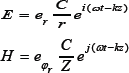
Where z is that the direction of propagation and r and z area unit cylindrical coordinates targeted on axis of the cable. Z is that the wave electric resistance within the non-conductor of the cable [2], associate in Nursing d C is a whimsical constant. The angular frequency is denoted by «. The propagation constant, k, relates to the wavelength within the medium λ as

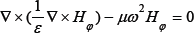
In the air, the electrical field conjointly incorporates a finite axial part whereas the flux is solely angle. So it's doable to model the Associate in Nursingtenna victimization an axisymmetric transversal magnetic (TM) formulation, and also the differential equation becomes scalar in Hq:

Figure 1: The pure mathematics of the antenna.

The antenna pure mathematics consists of a 0.2m tall bronze cone with a prime angle of ninety degrees on a finite ground plane of a 0.282m radius. The concentrically feed incorporates a central conductor of 1.5millimetre radius Associate in nursing an outer conductor (screen) of 4.916millimetre radius separated by a Teflon non-conductor of relative permittivity of 2.07. The central conductor of the cable is connected to the cone, and also the screen is connected to the bottom plane. The model takes advantage of the motion symmetry of the matter, which permits modeling in 2nd victimization cylindrical coordinates (Figure 1). You'll be able to then use a really fine mesh to attain a superb accuracy. The central conductor of the cable is connected to the bronze cone, and also the cable screen is connected to the finite ground plane.

Designing a biconical antenna using comsol tool [3], to generate the above biconical antenna geometry we needed the following steps:

Figure 2: Rectangle with dimension length of 28.2cm.

A. First we draw a rectangle 1 with width 28.2 and height dw i.e. 30.1cm as shown in above Figure 2.

B. Then we draw a rectangle 2 with width 0.342 and height 10cm, adjacent to the rectangle 1 as shown in above Figure 3 in blue color.

Figure 3: Rectangle 2 with dimension length of 0.342cm.

C. Then we draw a rectangle 3 with width 27.6 and height 9.1cm, adjacent to the rectangle 2 as shown in above Figure 4.

D. By using r=0.3, 0.3, 0.15, 0.065, 0.1, 0.0015 and z=0, 0.2, 0.2, 0.1, 0.1, 0 we design a polygon as shown in blue in Figure 5.

E. Symmetrical half of typical biconical antenna is shown in Figure 6. The central conductor of the cable is connected to the bronze cone, and also the cable screen is connected to the finite ground plane.

Figure 4: Rectangle 3 with dimension length of 27.6cm.

Figure 5: Polygon design.

Figure 6: Symmetrical half of biconical antenna.

F. Symmetrical half of novel biconical antenna is shown in Figure 7. The central conductor of the cable is connected to the bronze stepped cone, and also the cable screen is connected to the finite ground plane.

Figure 7: Symmetrical half of novel biconical antenna.

G. Then a semi-circle of radius of 60cm is drawn as an air domain for radiation pattern which is shown in Figure 8.

Figure 8: Symmetrical half of novel biconical antenna.

Appling material

Figure 9: Appling material.

The central conductor of the cable is connected to the stepped cone is made up of bronze, and also the cable screen is connected to the finite ground plane (Figure 9). The concentrically feed incorporates a central conductor of 1.5 millimetre radius Associate in nursing an outer conductor (screen) of 4.916millimetre radius separated by a Teflon non-conductor of relative permittivity of 2.07 [4]. The central conductor of the cable is connected to the cone, and also the screen is connected to the bottom plane (Table 1).

Table 1: Teflon properties.

Boundary conditions

By using Electromagnetic Waves, Frequency Domain physics we can analyze the novel stepped biconical antenna. The boundary conditions for the bronze surfaces are:

Figure 10: Boundary conditions for the bronze surfaces.

Figure 11: Meshing.

At the feed purpose, a matched concentrical port stipulation is employed to form the boundary clear to the wave. The antenna is divergent into free area, however you'll be able to solely discretize a finite region. Therefore, truncate the pure mathematics a long way from the antenna employing a scattering stipulation providing outgoing spherical waves to pass with little reflections [5]. A symmetry stipulation is mechanically applied on boundaries at r=0, as shown in Figure 10.

Meshing

By meshing we can interruption of the geometry into small parts to make the solution more accurate, as shown in Figure 11.

Figure 12: Appling frequency range.

Study

In study we provide the study parameters for geometry, in this model we apply the frequency at terminal ranging from 200MHz to 3GHz with a step size of 25MHz as shown in Figure 12.

Figure 13: Electric field basic.

Figure 14: Electric field of stepped.

In post processing we analyze the various results of the basic design and new proposed stepped biconical antenna design with various parameters of them [6].

Electric field

The electric field of basic biconical antenna are shown in Figure 13, the blue and red circles around the cone in air domain are shown, with maximum value of 118A/m. The electric field of proposed stepped biconical antenna are shown in Figure 14, the blue and red circles around the cone in air domain are shown, with maximum value of 89.6A/m.

Figure 15: S-parameter basic.

S-parameter

Figure 16: S-parameter of stepped.

The S-parameter of basic biconical antenna is shown in Figure 15, the losses in dB are shown for range of frequency is shown below with maximum loss of -12dB. The S-parameter of proposed stepped biconical antenna is shown in Figure 16, the losses in dB are shown for range of frequency is shown below with maximum loss of -21dB, which is nearly double of the basic biconical antenna [7].

Far-field norm (V/m)

Figure 17: Far field basic.

Figure 18: Far field of stepped.

The polar far field pattern of basic biconical antenna are shown in Figure 17, with band of frequency starting from 200MHz to 3GHz with step size of 25MHz. The polar far field pattern of stepped biconical antenna are shown in Figure 18, with band of frequency starting from 200MHz to 3GHz with step size of 25MHz. covers nearly double distance.

Far-field norm (V/m) 3D

The polar far field pattern of basic biconical antenna are shown in Figure 19, with band of frequency starting from 200MHz to 1.5GHz with step size of 25MHz. The polar far field pattern of stepped biconical antenna are shown in Figure 20, with band of frequency starting from 200MHz to 1.5GHz with step size of 25MHz a unique pattern of field is shown below [8].

In practice, the stepped biconical antenna is difficult to fabricate but the 10dB return loss result in the low frequencies is small compared to the normal biconical design. Thus the stepped biconical antenna may be useful in some applications which demand specific radiation pattern. The input impedance of the biconical antenna varies according to the step, as expected. It is observed that an optimum step exists for 50Ω matched impedance. From the above results, the influence of geometric parameters on impedance matching is noted. It is observed that the improvement in bandwidth can be obtained with the height of the biconical antenna is approximately equal dimension to the base radius of the cone.

Figure 19: Far field basic.

Figure 20: Far field of stepped.

1. WHO (2010) Global tuberculosis report 2010. Geneva, Switzerland.
2. Gillespie S (2008) Poverty, food insecurity, HIV vulnerability and the impacts of AIDS in sub-saharan Africa. IDS Bulletin 5(39): 10-18.
3. WHO (2014) Global tuberculosis report 2014, Geneva, Switzerland.
4. Nyirenda T (2007) Epidemiology of tuberculosis in malawi. Malawi Medical Journal 18(3): 147-159.
5. Kemp RJ, Mann G, Simwaka BN, Salaniponi FM, Squire SB (2007) Can malawi’s poor afford free tuberculosis services? patient and household costs associated with tuberculosis in LL. Bull World Health Organ 85(8): 580-585.
6. WHO (2013) Global Tuberculosis Report 2013. Geneva, Switzerland.
7. Collins TC, Henderson WH, Khuri FS (1999) Risk factors for prolonged length of stay after major elective surgery. Pub Med 230(2): 251.
8. Frietas A, Silva CT, Lopes F, Isabel GL, Armando TP, et al. (2012) Factors influencing hospital high length of stay outliers. BMC Health Services Research 12: 265.
9. Lee AH, Fung WK, Fu B (2003) Analyzing hospital length of stay: mean or median regression? Med Care 41(5): 681-686.
10. Atif M, Sulaiman SAS, Shafie AA, Asif M, Babar Z (2014) Resource utilization pattern and cost of tuberculosis treatment from the provider and patient perspectives in the state of Penang, Malaysia. BMC Health Serv Res 14(353).
11. McMullan R, Silke B, Bennett K, Callachand S (2004) Resource utilisation, length of hospital stay, and pattern of investigation during acute medical hospital admission. Postgrad Med J 80(939): 23-26.
12. Krell RW, Girotti ME, Dimick JB (2014) Extended length of stay after surgery: complications, inefficient practice, or sick patients? JAMA Surg 149(8): 815-820.
13. Hinchliffe SR, Seaton SE, Lambert PC, Draper ES, Field DJ, et al. (2013) Modeling time to death or discharge in neonatal care: an application of competing risks. Paediatr Perinat Epidemiol 27(4): 426-433.
14. Kim HT (2007) Cumulative incidence in competing risk data and competing risks regression analysis. Clin Cancer Res 13(2.1): 559-565.
15. Lim HJ, Zhang X, Dyck R, Osgood N (2010) Methods of competing risks analysis of end-stage renal disease and mortality among people with diabetes. BMC Medical Research Methodology.
16. Dignam JJ, Zhang Q, Kocherginsky MN (2012) The use and interpretation of competing risks regression models. Clinical Cancer Research Clin Cancer Res 18(8): 2301-2308.
17. Gooley TA, Leisenring W, Crowley J, Storer BE (1999) Estimation of failure probabilities in the presence of competing risks: New representations of old estimators. Statistics in Medicine 18(6): 695-706.
18. Hinchliffe SR, Seaton SE, Lambert PC, Draper ES, Field DJ, et al. (2013) Modeling time to death or discharge in neonatal care: an application of competing risks. Paediatr Perinat Epidemiol 27(4): 426-433.
19. Putter H, Fiocco M, Geskus RB (2007) Tutorial in biostatistics: competing risks and multi-state models. Stat Med 26(11): 2389-2430.
20. Koller MT, Raatz H, Steyerberg EW, Wolbers M (2011) Competing risks and the clinical community: irrelevance or ignorance? Stat Med 31(11- 12): 1089-1097.
21. Varadhan R, Weiss CO, Segal JB, Wu AW, Scharfstein D, et al. (2010) Evaluating health outcomes in the presence of competing risks: a review of statistical methods and clinical applications. Med Care 48(6 Supp): S96-S105.
22. Latouche A, Boisson V, Chevret S, Porcher R (2007) Mis-specified regression model for the sub-distribution hazard of a competing risk. Stat Med (26): 965-974.
23. Kleinbaum DG, Klein M (2005) Survival analysis, A self-Learning text. 2nd ediyion, Springer Science and Business media, New York, USA.
24. Aban I (2014) Time to event analysis in the presence of competing risks. Journal of Nuclear Cardiology 22(3): 466-467.
25. Gray RJ (1988) A class K-sample tests for comparing the cumulative incidence of a competing risk. Annals of Stat 16(3): 1141-1154.
26. Fine JP, Gray RJ (1999) A proportional hazards model for the subdistribution of competing risks. Journal of American Statistical Association 94(446): 496-509.
27. Jung JH, Fine JP (2007) Parametric regression on cumulative incidence function. Biostatistics 8(2): 184-196.
28. Borrebach DJ (2013) Comparisons between the kaplan meier complement and the cumulative incidence for survival prediction in the presence of competing events. Statistics, Pittsburgh, USA.
29. Sherif BN (2007) A comparison of kaplan-meier and cumulative incidence estimate in the presence or absence of competing risks in breast cancer data. Pittsburgh: Public Health, University of Pittsburgh, USA.
30. Roberts MS, Daley K (2003) A national study of clinical and laboratory factors affecting the survival of patients with multiple drug resistant tuberculosis in the UK. Thorax 9(57): 810-816.
31. Teixeira L, Rodrigue A, Carvalho MJ, Cabriata A, Mendonca D (2013) Modelling competing risks in nephrology research: an example in peritoneal dialysis. BMC Neohrology 14: 110.
32. Oliveira HMMG, Brito RC, Kritski AL, Ruffino NA (2009) Epidemiological profile of hospitalized patients with TB at a referral hospital in the city of Rio de Janeiro, Brazil. J Bras Pneumol 35(8): 780-787.