Adjusted Risk Difference Estimation: An Assessment of Convergence Problems with Application to Malaria Efficacy Studies

In Randomized Controlled Trials (RCTs), treatment effect for binary outcomes is usually measured using a risk ratio, an odds ratio or a risk difference [1]. Risk differences are becoming more widely reported in RCTs, especially in malaria efficacy studies [2-4]. These are now frequently used when the objective is to compare treatment effect between treatments as commonly used alternatives such as odds ratios and risk ratios can be difficult for general medical researchers to interpret [5]. A major concern with odds ratios is that these are prone to misinterpretation even when the efficacy of the outcome measure is common, easily leading to invalid inferences of treatment effect [6-9]. Likewise, risk ratios can be difficult to understand, especially in equivalence studies, as their interpretation depends on whether a failure or a success is being modelled; while failure and success rates are clearly complementary, the inference that can be drawn for each of these endpoints may differ in some cases [5,10].

Risk difference estimation is preferred by many researchers not only because it is easier to interpret but for the arguably more important reason that it is frequently the most relevant and biologically sensible measure to report [11] and provides a clear interpretation of the scientific question of interest. That is, it directly answers the question of whether there is a difference in risk and/or efficacy between two groups.

The binomial regression model with an identity link function is often the standard model used to estimate risk differences. Risk difference models, however, sometimes encounter the problem that the binomial regression algorithm fails to converge or to produce output [10]. The current literature suggests that this problem is most likely to occur when one or both rates are close to a boundary (0% or 100%) and hence when risk ratios approach either infinity or zero [12,13]. Experience working with risk difference modelling using the Stata software, however, shows that these models can sometimes fail to converge or produce output even in instances where both rates are reasonably distant from boundary values. Furthermore, even in scenarios when one or both rates are close to a boundary, convergence is can be achieved in some cases. These observations suggest that factors other than boundary problems may influence non-convergence and/or output failure.

Simulation studies were performed to evaluate the potential impact of convergence problems on the estimation of treatment effect using risk difference modelling when adjusting for potential confounders. This research was motivated by a malaria efficacy study that was conducted in Malawi between 2003 and 2005; full details of the methods and findings of this study are available in Bell DJ et al. [2] but to summarise briefly:

A four-group blinded randomized controlled study was performed to compare the efficacy of three Sulfadoxine- Pyrimethamine (SP)-Based Combination therapies (SP plus chloroquine (CQ), SP plus artesunate (ART) and SP plus amodiaquine (AQ)) plus a placebo (control) group. This control arm comprised of SP plus placebo as SP was the standard first line treatment for uncomplicated falciparum malaria in Malawi during the study period. The study was conducted in response to accumulating evidence indicating that some resistance to SP was developing, and because the WHO was recommending the use of combination therapies (especially the artemisinin combination therapies (ACTs)). Participants were children aged 1-5 years.

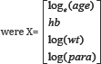
Treatment effect was modeled using risk differences. Covariates, denoted as X, included in the analyses

Adjusted risk difference modelling, however, encountered model failure problems.

Simulation studies were carried out to explore the impact of the following issues on model convergence rates: 1) the number of covariates in the model; 2) the level of correlation between the covariates; 3) the proximity to a boundary of one or more efficacies.

Datasets were simulated based on the methods and results of the randomized control trial described in the previous section Bell et al. [2]. These were used to compare the efficacy rates in two treatment groups ("active" and control) with adjustment for up to two covariates. Two patterns of correlation between the covariates were examined; no/negligible correlations and correlations similar to those found by Bell et al. [2]. All simulations used a sample size 200 (100 participants randomized to each group), again as used by Bell et al. [2]. Five thousand (5,000) datasets were simulated for each scenario considered. Independent (predictor) variables were generated using multivariate log-Normal distributions except for haemoglobin level (hb) which was generated using a Normal distribution; these were used as covariates in a binomial model using an identity link to estimate the risk difference between the treatment and control arms.

The choice of covariates was based on expert knowledge from malaria researchers suggesting that age, weight (wt), haemoglobin (hb) level and parasite count (para) can confound the relationship between treatment and efficacy in malaria RCTs. Standard practice in such RCTs is to estimate adjusted treatment effects controlling for potential confounders.

Parameter values for simulation of covariates

The matrices of parameters and values for simulating the baseline covariates were as follows:

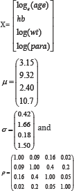
X is a vector of values for the four covariates: log(age), log(wt), log(para) and haemoglobin (hb).

μ and σ are vectors of mean and standard deviation values respectively for (in order) log(age), hb, log(wt) and log(para).

ρ is a matrix of correlations among the four covariates.

Randomization

The simulated pre-study covariate observations were randomly allocated to two treatment groups, A and B, in the ratio 1:1 using blocks of size 10.

Simulation of a binary outcome variable

After randomization of the simulated observations, the outcome measure (1=success, 0=failure) was generated for each of the two groups to achieve the required efficacy (treatment success) rates using a Bernoulli (π_i) distribution, where π_i is the mean proportion of subjects with treatment success (efficacy) in a group i (i=A,B). This resulted in a simulated binary outcome variable with group success (efficacy) and failure rates of π_i, and 1-π_i respectively. The simulations were constrained to ensure that the specified rates were achieved exactly.

The risk difference model can be fitted in the Generalized Linear Model (GLM) framework. A GLM is constructed using three statistical functions: the linear function, the link function and the variance function [12,13]. The linear function may be parameterized as follows:

ø_i = β₀ + β₁ x_1i +........β_px_pi

where x_pi is the p^th covariate or factor for individual i and (β₀, β₁ β_p) is a vector of regression coefficients.

The link function is specified as: g^(E(Yi⁾⁾ = ø_i that is, the link function describes how the expected value of the outcome variable E(Y)depends on the linear predictor ø_i. Note that g^(E(Yi⁾⁾ can be specified either as the identity function (no transformation on the E(Y)), or as a logit, log, log-binomial etc. along with a relevant family such as Poisson, Binomial, Gaussian and Gamma.

Finally, the variance function is given by var(Y_i) = φV(E(Y)), where φ is a constant, commonly referred to as a dispersion parameter

The outcome variable Y_i. follows a binomial distribution denoted by y_i~Binomiai(n_i,π_i), where n_i and π_i are the number of participants and treatment efficacy rate respectively in group i.

The main interest is to model the probability of a treatment success (efficacy) y / n in the form of a risk difference model, where:

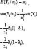
So the variance function v ð_i,(is ð_i) - _i which is a function of E(Y_i / n_i), and the dispersion parameter is &x966; = 1 / n_i.

Estimates of the risk differences are obtained by specifying an identity link function to the binomial regression model. The coefficients in the Binomial regression model with identity link produce risk differences as follows:

Consider what happens when a variable X is increased by 1 unit.

P(Y = 1|X) = X β , where Y=1 denote treatment success and Y=0 denote treatment failure.

P(Y = 1| X+1) = (X + 1)β .

X can be thought of as a reference group and X+1 as a treatment group of interest. Taking the difference gives:

P(Y = 1/X + 1) - P(Y = 1/X) = (X + 1)β - (x)β= β, which is a risk difference.

In the multivariable model P(Y=1/x₁,x₂,....x_p) = β₀ +β₁X_1i +β₂X_2i+......β_pX_pi the regression coefficients β_pi represent the risk difference resulting from a change (increase) of one unit in the explanatory variable X_pi. When using the identity link, fitted probabilities outside the probability range (0,1) are possible. Wacholder [11,13] suggested that when fitting a binomial regression model with identity link, the fitted probabilities should be checked for range conditions at each iteration. If found to be outside the permitted range, then they should be reset it to be within that range.

Risk difference models considered in this study included subsets of between one and three of the continuous covariates age, wt, para or hb, and a binary factor taking values of 1/0 indicating treatment given/not given.

Correlations and number of covariates included in modelling

In the first set of simulations, the contributions to binomial regression model convergence rates due to the (i) the proximity of efficacy rates to boundary vales and (ii) the number of covariates were assessed using correlation levels between the covariates reflecting those observed in the sample dataset. The efficacy rate in one group was allowed to approach a boundary (100% in this case) while that in the other group was held constant. For example, in one group efficacy was set at 60% and in the other group it was varied to take values 70%, 80%, 85% or 90%, and convergence rates were estimated in each scenario.

To assess the impact of level correlation between covariates on the ability of models to converge, the pair wise correlations between the covariates were reduced to zero and the same models fitted while monitoring convergence. In these simulations, for each pre-set risk difference, the number of covariates and the correlation levels were varied.

Statistical software

All simulations were performed using Stata 12.0, IC, StataCorp, 4905 Lakeway Drive, College Station, Texas 77845 USA. Graphs were constructed using Microsoft Excel 2007.

Effect of proximity to boundary of efficacy levels and number of covariates on convergence of a binomial regression model

When using just a single predictor variable (covariate) and with the efficacy levels set at 60% and 70% for the two groups respectively (i.e. distant from the boundary of the parameter space), the percentage of datasets that converged when a binomial regression model was fitted was high (96.8% to 99.7%) (Table 1); however, while the corresponding non-convergence rates were very low, they were not negligibly so.

Table 1: Convergence rates by efficacy rate and number of covariates in model (averaged over 5000 simulated datasets-correlated).

Convergence rates remained high, ranging from 92.0% to 94.7%, even when the larger of the two efficacy levels were increased to 85%. However, when the larger efficacy level was increased to 90% (still some distance from the boundary), convergence levels dropped dramatically between 81.3% and 86.6%.

Adding additional covariates exacerbated this problem. With the larger of the two efficacy levels set at 90%, convergence was obtained in 59.8% to 66.1% of models involving two covariates, and in only 42.9% to 48.1% of models involving three covariates. The full extent of this trend is shown graphically in Figure 1.

Figure 1: Percentage convergence by efficacy rates and correlation structure.

The effect of correlations between covariates on model convergence

The influence of correlation levels on model convergence rates was examined for efficacy rates of 60% and 85% in the two groups respectively (Table 2 and Figure 2). In these simulations, the impact of setting the correlations between each pair of covariates to zero was compared to that obtained using the correlation levels from the original RCT.

Table 2: Convergence rates in the presence and absence of correlation between covariates (averaged over 5000 simulated datasets): efficacy rates 60% and 85%.

Figure 2: Effect of reducing correlation on convergence (efficacy rates: 60% and 85%).

For all models considered, the convergence percentage improved when the correlations between covariates were removed. The improvement in convergence rates increased as the number of covariates in the model was raised.

For many researchers, risk difference is increasingly the preferred measure of treatment effect in RCTs and in epidemiological cohort studies where the primary outcome measure is dichotomous. Estimating risk differences adjusted for important covariates can be problematic, however, due to the problem of the binomial regression model failing to converge. This simulation study found that non-convergence rates tend to rise as the number of continuous covariates included in the model increases, as correlation levels between covariates increase, and (most severely) when efficacy rates in either treatment arms is close to a boundary (i.e. to 0% or 100%).

When using maximum likelihood estimation, as is frequently the case with binomial regression models, software algorithms may fail to converge either because of poor starting values for the iterative computing process (e.g. starting values not in the restricted parameter space) or because the maximum likelihood solution occurs on the boundary of the parameter space [12]. The first of these causes can be fixed easily by specifying better starting values. In the latter situation, however, the derivative of the likelihood at its maximum may not be 0 (in which case standard software packages that maximize the likelihood by finding the point at which the derivative is equal to 0 (namely Newton's method), may be unable to find a solution) or could be a result of having a flat likelihood distribution.

In summary, binomial model non-convergence rates were found to increase as efficacy rates in one or both treatment groups moved towards a boundary value irrespective of the number of covariates included in the model. Indeed, it is interesting to note that the problem worsened as the number of covariates in the model increased and as the efficacy rate in either treatment group moved towards a boundary value. That is, models with just one covariate had less convergence problems than models with two covariates, and in turn these had fewer convergence problems than models with three covariates.

For all scenarios examined, convergence was poor when the efficacy rate in either group was 90% or greater. Additionally, nonconvergence rates increased with increasing levels of correlation between any covariates included in the model.

This work was supported by the European and Developing Countries Clinical Trials Partnership (EDCTP) grant number IP.2007.31060.03; and the Johns Hopkins University Center for AIDS Research (Grant Number1P30AI094189) from the National Institute of Allergy And Infectious Diseases.

1. Magder LS (2003) Simple approaches to assess the possible impact of missing outcome information on estimates of risk ratios, odds ratios, and risk differences. Control Clin Trials 24(4): 411-421.
2. Bell DJ, Nyirongo SK, Mukaka M, Zijlstra EE, Plowe CV, et al. (2008) Sulfadoxine-pyrimethamine-based combinations for malaria: a randomised blinded trial to compare efficacy, safety and selection of resistance in Malawi. PLoS One 3(2): 1578.
3. Arinaitwe E, Sandison TG, Wanzira H, Kakuru A, Homsy J, et al. (2009) Artemether-lumefantrine versus dihydroartemisinin-piperaquine for falciparum malaria: a longitudinal, randomized trial in young ugandan children. Clin Infect Dis 49(11): 1629-1637.
4. Mukaka M, White SA, Mwapasa V, Kalilani PL, Terlouw DJ, et al. (2016) Model choices to obtain adjusted risk difference estimates from a binomial regression model with convergence problems: An assessment of methods of adjusted risk difference estimation. Journal of Medical Statistics and Informatics 4: 5.
5. Mukaka M, White SA, Terlouw DJ, Mwapasa V, Kalilani PL, et al. (2016) Is using multiple imputation better than complete case analysis for estimating a prevalence (risk) difference in randomized controlled trials when binary outcome observations are missing? Trials 17: 341.
6. Case LD, Kimmick G, Paskett ED, Lohman K, Tucker R (2002) Interpreting measures of treatment effect in cancer clinical trials. The Oncologist 7(3): 181-187.
7. Davies HT, Crombie IK, Tavakoli M (1998) When can odds ratios mislead? BMJ 316(7136): 989-991.
8. Page J, Attia J (2003) Using Bayes' nomogram to help interpret odds ratios. ACP J Club 139(2): A11-A12.
9. McNutt LA, Wu C, Xue X, Hafner JP (2003) Estimating the relative risk in cohort studies and clinical trials of common outcomes. Am J Epidemiol 157(10): 940-943.
10. Cheung YB (2007) A modified least-squares regression approach to the estimation of risk difference. Am J Epidemiol 166(11): 1337-1344.
11. Walter SD (2000) Choice of effect measure for epidemiological data. J Clin Epidemiol 53(9): 931-939.
12. Deddens JA, Petersen MR (2008) Approaches for estimating prevalence ratios. Occup Environ Med 65(7): 481-506.
13. Wacholder S (1986) Binomial regression in GLIM: estimating risk ratios and risk differences. Am J Epidemiol 123(1): 174-184.