Cancer, Quantum Computing and TP53 Tumor Suppressor Gene Mutations Prediction

Introduction

For more than 25 years, we have been looking for bio mathematical laws controlling and structuring DNA, genes, proteins, chromosomes and genomes [1,2]. In 1997 we discovered a simple numerical law based solely on atomic masses, UNIFYING the 3 languages of biology: DNA, RNA, and amino acids. This law, “the MASTER CODE OF BIOLOGY” is published in 2009 in the book CODEX BIOGENESIS [3] and then in 2015 in a reference article peer review [4]. In 2017 we publish different applications: HIV, SNPs, brain genetics: Prions, Amyloids, DUF1220 [5-10].

In other hand, the TP53 Tumor Suppressor gene plays a central role in a majority of cancers [11,12]. Between January 1993 and July 1996, more than 4300 papers have been published in which the term “p53” appears in the title! This massive interest in a single protein is almost unprecedented and reflects the central place of p53 in the regulation of cell number and the frequency with which abnormalities of p53 occur in human tumors. P53 has been named Molecule of the Year by the editors of the journal Science [13], and the “guardian of the genome” by many researchers.

Somatic TP53 mutations occur in almost every type of cancer at rates from 38% - 50% in ovarian, esophageal, colorectal, head and neck, larynx, and lung cancers to about 5% in primary leukemia, sarcoma, testicular cancer, malignant melanoma, and cervical cancer [11].

The mutations of TP53 are well known and listed, classified according to their frequencies and the types of cancers involved in these mutations [12]. Based on studies that examined the whole coding sequence, 86% of mutations cluster between codons 125 and 300, corresponding mainly to the DNA binding domain.

The results - never published - that will be presented here were obtained in 2001 from the IARC TP51 mutations data banks available around that time [12].

Methods

Master code summary

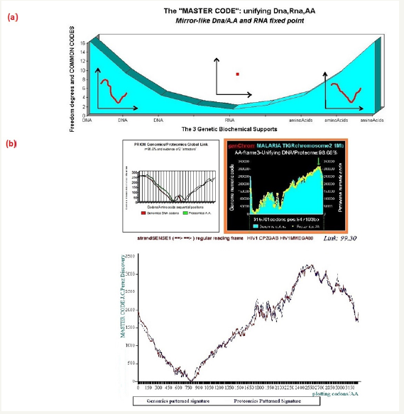
Starting from the atomic masses constituting nucleotides and amino acids, a numerical scale of integers characterizing each bioatom, each TCAG DNA base, each UCAG RNA base, or each amino acid, an integer numbers scale code is obtained. Then, for each sequence of double - stranded DNA to be analyzed, the sequence of integers that characterizes it (genomics) is constructed as well as the sequence of amino acids that would encode this double strand if each of the strands was a potential protein (proteomics). The remarkable fact is that this proteomics image still exists, even for regions not translated into proteins (junk dna). The computational methodology of the Master code [3,4] then produces 2 patterned images (2D curves, Figure 1) which are very strongly correlated. This would mean that beyond the visible sequence of DNA there would be a kind of MASTER CODE being manifested by two supports of biological information: the sequences of DNA and of amino acids, the RNA image constituting a kind of neutral element like the zero of the mathematics. Our thousands of genes and genomes Master Code analyses (viruses, archaeas, bacteria, eucharyotes) demonstrated that the extremums (max and min) signify functional regions like proteins activeites, fragility points like chromosomes breakpoints) (Figure 1).

Figure 1: Master code of biology” and Great Unification shows an equivalence of both Genomics (DNA) and Proteomics (amino acids) signatures while the RNA signature is a neutral area like a “zero”. (b) A typical correlation between Genomics and Proteomics signatures related to the Prion protein, the whole Malaria chromosome 2, and the whole HIV1 genome.

Detailing the master code computing

A quick presentation of the formula for life: In [3,4] we introduced the law we call Formula for Life. This law unifies all of the components of living including bio-atoms, CONHSP and their various isotopes, to genes, RNA, DNA, amino acids, chromosomes and whole genomes. This law is the result of a simple non-linear projection formula of the atomic masses. The result of this projection is then organized in a linear scale of integer number based codes (e.g., -2, -1, 0, 1, 2, 3...) coding multiples Pi/10 regular values. These codes are called Pi-masses.

The result is a real number which we retain only the residues (decimal remainder). Detailing the “PPI (mass)” projection: Consider any atomic mass « m », which may be that of a bio-atom, of a nucleotide, of a codon, of an amino acid or of other genetic compound based on bio-atoms or even, any atoms (Mendeleiëv Table 1), [14]).

Pr ojPPI (m) = [1−[ pΠ]]m

Where, P = 0.742340663...

This process will work especially on the average masses (Table 1). But it may also be applied to a particular isotope or any derivative of specific atomic mass proportions of the various isotopes (Table 1).

An Overview on the “Biology Master Code” Great Unification of DNA, RNA and Amino Acids

It may seem surprising that such a fine tuned process like biology of Life requires the use of three languages as diverse and heterogeneous as DNA with its alphabet of four bases TCAG; RNA with its alphabet of four bases UCAG; and proteins with their language of 20 amino acids. Obviously, the main discoveries in biology were made by those who managed to unearth the respective areas and “bridges” between these three languages. However, any “aesthete” researcher will think the table of the universal genetic code seems rather “ad hoc” and heterogeneous.

Table 1: Example of Pi-mass projection fine-tuned selectivity for Oxygen average mass vs. individual isotopes.

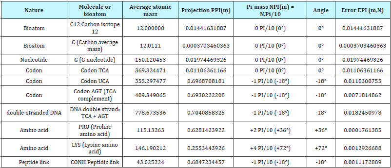
Notes: Projections PPI (m) are multiples of Pi:10. Example: 0.314... = 1Pi/10, 0.628... = 2Pi/10, etc... But, symmetrically vs. 0Pi/10, it appears another regular scale of attractors in the negative region of Pi/10: -1Pi/10 = 1-0.314 = 0.685..., -2Pi/10 = 1-0.628.

Starting only from the double-stranded DNA sequence data, the “Master Code” is a digital language unifying DNA, RNA and proteins that provide a common alphabet (Pi-mass scale) to the three fundamental languages of Genetics, Biology and Genomics.

The construction method of “the Master Code” will be now fully described below. It will highlight a significant discovery we summarize as follows: “Above the 3 languages of Biology - DNA, RNA and amino acids, there is a universal common code that unifies, connects and contains all these three languages”. We call this code the “Master Code of Biology.”

Here is a Brief Description of our Process for Computing the Master Code

The coding step: First, we apply it to any DNA sequence encoding a gene or any non-coding sequence (formerly mislabelled as junk DNA). So it may be either a gene, a contig of DNA, or an entire chromosome or genome. In this sequence, we always consider double-stranded DNA as we explore the following three codon reading frames and following the two possible directions of strand reading (3’ ==> 5’ or 5’ ==> 3’). The base unit will always be the triplet codon consisting of three bases.

As shown in above sample, we calculate the Pi-mass related to double stranded triplets DNA bases, double stranded triplets RNA bases, and double-stranded pseudo amino acids. In fact, for each DNA single triplet codon, we deduce the complementary Crick Watson law bases pairing. We do the same work for RNA pseudo triplet codon pairs, then, similarly for amino acids translation of these DNA codon couples using the Universal Genetic Code table. Then, we obtain 3 samples of pairs codes: DNA, RNA and amino acids and this, systematically even when this DNA region is genecoding or junk-DNA.

A simple example: the starting region of prion gene

DNA image coding:

ATG CTG GTT CTC TTT...

-1 -1 -1 0 0...

Complement:

TAC GAC CAA GAG AAA...

0 -1 0 -2 0...

RNA image coding:

AUG CUG CUU CUC UUU...

-2 -2 -3 -1 -3...

Complement:

UAC GAC GAA GAG AAA...

-1 -1 0 -2 0...

Proteomics image coding:

MET LEU VAL LEU PHE

4 3 3 4 3...

Complement:

TYR ASP GLN GLU LYS

2 -1 1 0 4...

Pi-masses corresponding to two strands are then added for each triplet:

Double strand DNA image coding: -1 -2 -1 -2 0...

Double strand RNA image coding: -3 -3 -3 -3 -3...

Double strand Proteomics image coding: 6 2 4 4 7...

This produces three digital vectors relating to each of the 3 DNA, RNA, and proteomics coded images. At this point we already reach an absolutely remarkable result, as symbolized in Figure 1.

We will focus now - exclusively - on the DNA code (genomics) and amino acids code (proteomics).

The globalization and integration step

To these two numeric vectors we apply a simple globalization or integration linear operator. It will “spread” the code for each position triplet across a short, medium or long distance, producing an impact or “resonance” for each position and also on the most distant positions, reciprocally by feedback. This gives a new digital image where we retain not the values but the rankings by sorting them.

We run this process for each codon triplet position, for each of the three codon reading frames and for the two sequence reading directions (3’ ==> 5’ and 5’ ==> 3’).

For example, to summarize this method: on starting area of the GENOMICS (DNA) code of Prion above, the “radiation” of triplet codon number 1 would propagate well:

-1 -2 -1 -2 0... ==>

-1 -3 -4 -6 -6...then, we cumulate these values: -20

So we made a gradual accumulation of values.

The same operation from the codon number 2 produces:

-1 -2 -1 -2 0... ==>

-2 -3 -5 -5...then, we cumulate these values: -15

etc.

Similarly, the same process on starting area of the PROTEOMICS code of Prion above, the “radiation” of triplet codon number 1 would propagate well:

6 2 4 4 7... ==>

6 8 12 16 23...then, we cumulates these values: 65

So we made a gradual accumulation of values.

The same operation from the codon number 2 produces:

6 2 4 4 7... ==>

2 6 10 17...then, we cumulate these values: 35

etc.

Finally, after computing by this method these “global signatures” for each codon position at Genomics and Proteomics levels, we sort each genomic and proteomic vector to obtain the codon positions ranking: example: as illustrated bellow, the Genomics ranking patterned signature is 2 1 4 3 5 for this Prion starting 5 codons mini subset sequence of 5 codons positions (arbitrary values). Then, to summarize the Master Code computing method on these 5 codon positions starting Prion protein sequence:

Genomics signature:

Codon 1:

Codon / Basic codes / Potentials (with circular closure) / circular complements:

!

-1 -2 -1 -2 0

-1 -3 -4 -6 -6

0

Cumulates: -20

Codon 2:

Codon / Basic codes / Potentials (with circular closure) / circular complements:

!

-1 -2 -1 -2 0

-2 -3 -5 -5

-6

Cumulates: -21

Codon 3:

Codon / Basic codes / Potentials (with circular closure) / circular complements:

!

-1 -2 -1 -2 0

-1 -3 -3

-4 -6

Cumulates: -17

Codon 4:

Codon / Basic codes / Potentials (with circular closure) / circular complements:

!

-1 -2 -1 -2 0

-2 -2

-3 -5 -6

Cumulates: -18

Codon 5:

Codon / Basic codes / Potentials (with circular closure) / circular complements:

!

-1 -2 -1 -2 0

0

-1 -3 -4 -6

Cumulates: -14

Final rankings:

Codon positions: 1 2 3 4 5

Potentials: -20 -21 -17 -18 -14

Rankings: 2 1 4 3 5

Then we run similar computing for Proteomics...

Codon 1:

Codon / Basic codes / Potentials (with circular closure) / circular complements:

!

6 2 4 4 7

6 8 12 16 23

0

Cumulates: 65

Codon / Basic codes / Potentials (with circular closure) / circular complements:

!

6 2 4 4 7

2 6 10 17

23

Cumulates: 58

Codon 3:

Codon / Basic codes / Potentials (with circular closure) / circular complements:

!

6 2 4 4 7

4 8 15

21 23

Cumulates: 71

Codon 4:

Codon / Basic codes / Potentials (with circular closure) / circular complements:

!

6 2 4 4 7

4 11

17 19 23

Cumulates: 74

Codon 5:

Codon / Basic codes / Potentials (with circular closure) / circular complements:

!

6 2 4 4 7

7

13 15 19 23

Cumulates: 77

Final rankings:

Codon positions: 1 2 3 4 5

Potentials: 65 58 71 74 77

Rankings: 2 1 3 4 5

Then finally:

Codon position: 1 2 3 4 5

Genomics vector: 2 1 4 3 5

Proteomics vector: 2 1 3 4 5

To complete, the same work must be also operate on each codon reading frame...

Meanwhile, a more synthetic means to compute these “long range potentials” for each codon position is the following formula:

Cumulate potential of codon location “i”

P(i) = np(i) + [(n −1).p(i +1)] + [(n − 2).p(i + 2)]....+ [(n −1(n −1)).p(i + (n −1))]

Then finally,

P(i) = FORj = [0,(n −1)] DOSIGMA+ [(n − J ).p(i + j)]

Example for Genomics image of codon “i”

The initial computing method described above provides:

-1 -2 -1 -2 0... ==>

-1 -3 -4 -6 -6...then, we cumulate these values: -20

Becomes, using this new generic formula:

(−1)×5 + (−2)× 4 + (−1)×3+ (−2)× 2 + (0)×1 = (−5) + (−8) + (−3) + (−4) + 0 = −20

The Great Unification between Genomics and Proteomics Master Code Images

When applying the process described above in any sequence – gene coding, DNA contig, junk-DNA, whole chromosome or genome - a second surprise appears just as stunning as that of RNA neutral element. We find that for one of the three reading frames of the codons given, the Genomics patterned signature and the Proteomics patterned signature are highly correlated.

Contrary to the three genomics signatures which are correlated in all cases, the proteomics signatures are correlated with genomics signatures only for one codon reading frame, and generally in dissonance for the two remaining codon reading frames. Also, there are perfect local areas matching’s focusing on functional sites of proteins, hot-spots, chromosomes breaking points, etc.

Figure 1 summarizes this universal breakthrough for the general case and for three representative cases: Prion protein [10], a whole chromosome of Malaria disease, and a complete HIV1 genome [5]. It is important to note the universal character of this coupling of genomics/proteomics: for example, for some three billion base pairs of the whole human genome, we have verified this law across the entire genome, for all its chromosomes and in all its regions with a global correlation of about 99%.

In this global correlation, specific codon positions were a perfect match. This is remarkable when regions correspond to biologically functional areas: hot-spots, the active sites of proteins, breakpoints and chromosome fragility regions (i.e., Fragile X genetic disease), etc.

Gen lights

A method for mapping regions of mutability of a gene.

Our Master Code basic research output could predict the MUTABILITY level of each codon value and position relating to its effect at the whole structure level of the Genomics/Proteomics Unification data.

Then, we could associate with each codon position a “MUTABILITY COEFICIENT” varying from 1 to 61:

1 if the codon is the best by 61 possible values (without STOP codons values).

61 if any codon change increases the global Genomics/ Proteomics coupling ratio of the whole gene.

We note that low coefficient region correspond with optimal and “CONSERVED” regions.

Contrarly, high coefficient regions correspond with high MUTABILITY experimentally observed regions.

Then to summarize, in the case of gene = p53 long of 393 amino acids,

For each codon position « i » from i = 1 to 393,

DO: build 61 pseudo sequences where gene (i) = each possible coding codon

Compute scores = 61 Master Code methods (gene (i))

Compute score (real codon i) = score of the real codon i in the hierarchy of 61 scores (i).

Final result is an array of 393 scores with values between 1 and 61. Low values codon scores near 1 reveals conserved optimal codons related to a good Master Code coupling ratio.

Contrarly, high values codon scores near 61 reveals bad Master Code coupling rato, then probably a high potential mutagen codon location Figure 4.

Results and Discussion

The P53 is a 393 amino acids proteins coming from a long 20k bases length 11 exons gene from the chromosome 17p13. The P53 protein has 5 blocks of highly conserved regions at residues 117-142, 171-181, 234-258 and 270-286. These highly conserved regions coincide with the mutation clusters and HOTSPOTS found in p53 in human cancers, most of which have been found within exons 5 - 8. These mutations have been found to be highly frequent at the four mutational “hotspots” at codons 175, 245, 248 and 273.

In The following Figure 2, Cho Y et al. illustrate the complex interaction provided between P53 and DNA molecule: (Figure 2).

Figure 2: p53 interacting with DNA. Method: X-ray diffraction. [See Cho Y et al. for details!].

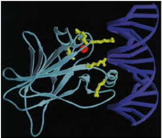
“The DNA (blue) and core domain (turquoise) are shown with the zinc atom (red), with the position of the six hot spot amino acid residues (yellow). Mutations in hot spot amino acids either interfere with protein-DNA contacts, or disrupt integrity of the domain. Thus, all naturally occurring mutations in p53 directly or indirectly affect the interaction of p53 with DNA, demonstrating that sequencespecific DNA binding is central to the normal functioning of p53 as a tumour suppressor.”

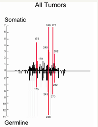
In other hand, these HOTSPOTS mutations are present in all kinds of CANCERS (Figure 3).

Figure 3: P53 mutations are very well referenced in databases [11,12].

Then, what about the PREDICTION of these MUTATIONS by our theoretical predictive method? (Figure 4)

Figure 4: Predicting individual codons mutability potential in TP53 tumor suppressor.

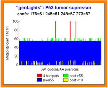
All codons positions are affected by a MUTABILITY COEFFICIENT in the range of 1 to 61:1 signify that this real codon value is the optimal one possible. 61 signify that any mutation on this position increases the global Genomics/Proteomics organization of the gene.

This kind of codons has then a high MUTABILITY power.

In the figure, we show (red) the four Hotspots codons positions 174 245 248 273.

Green bars illustrate high mutability codons (coef >55).

Contrarily yellow bars illustrate high conserved and optimal codons.

Then, the PREDICTION MUTABILITY SCORE COEFFICIENT of the 4 Hotspots is PERFECT:

Hotspot 175: coef=61 (the higher mutability possible level).

Hotspot 245: coef=61 (the higher mutability possible level).

Hotspot 248: coef=57 (very high mutability coef ie range 1-61).

Hotspot 273: coef=57 (very high mutability coef ie range 1-61) (Figure 4)

Below, in this other simulation run (Figure 5), we analyze the 622 GERMLINE single mutations reported in [15].

The Correlation between Experience and Prediction is Perfect

Horizontally, we represent all mutations sorted by decrease frequency values: on the left, high frequency mutations (codons 248 245 175 273). On the right, rare mutations points.

Simultaneously, the red bars represent the mutation effect on Genomics/Proteomics: on the left, this ratio increases, then on the right, this ratio decreases!

In blue, we plot the evolution of the mutability coef: high for frequent mutations, low or flat for others. Now, we have a good proof of the PREDICTION POWER of out Master Code based theoretical predictive mutagenesis method improved on the best example on MUTABILITY: P53, the “King Cancers gene” (Figure 5).

Figure 5: In 622 Germline mutations, we correlate predictive method and experimentaly observed mutations frequencies.

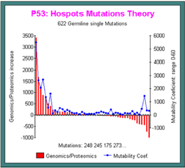
Figure 6: Major TP53 Hotspots “Islands mutations”.

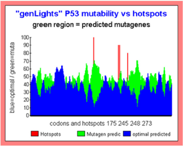
Other powerful representation of the “MUTABILITY GLOBAL SPACE” is the following.

In this kind of figures, we do a smoothing on the basic Master Code scores outputs. Then we compare patterns related with high mutability (green) with patterns related to low mutability (blue).

The superposition of both graphics provides “patterned ISLANDS”. Then green islands regions traduce a globally high MUTAGENE region. On the contrary, blue predominance regions corresponds with highly globally OPTIMAL region (then conserved).

In this graphics, we note that the four Hotspots are located in (or close) high global mutability regions. We see also, in the region of codons 80 an optimal region which must normally be highly CONSERVED (Figure 6).

Conclusion and Quantum Computing Considerations

The analysis that has just been presented here was performed on a simple PC computer and programmed with APL, a language more than fifty years old [16].

Prehistoric tools in the face of the quantum computer [17,18], but, nevertheless, APL is a language capable of manipulating objects of any mathematical dimension in parallel.

On the other hand, the results presented here were made almost 20 years ago (in 2000) but never published.

We will now discuss different avenues that reasonably suggest an implementation of this method on quantum computers.

Table 2: The Periodic Table of Biology” structuring ALL compounds of Life in a regular Pi/10 units scale.

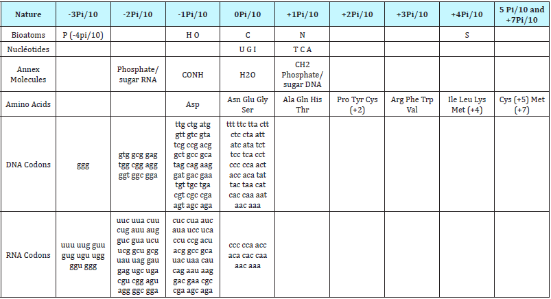
-2qubits will be enough to code the base pairs of the GENOMIC Code (2 * 2).

-4 qubits (2 * 4) will suffice to code the amino acid pairs of the PROTEOMIC Code.

- Finally the processes of Figures 4 & 6 are naturally parallel: we explore the Genomics and Proteomics master codes for each triplet codon the 64 possible values, ie 64 = 2 * 6 = 6 qubits.

Then, to conclude, the theoretical method of predicting mutagenic regions of TP53 is shown to be perfectly correlated with the mutagenic hotspots and codons referenced from thousands of cases of individual cancers observed (IARC database). It is likely

that this method is universal insofar as it can be applied to the prediction of mutagenic regions of any other gene, protein, human, animal or plant.

The parallel computation method described here can be generalized and then implemented in quantum computers in order to apply it to very long genes or even to entire chromosomes [19- 22].

References

1. Perez JC (1991) Chaos DNA and neuro-computers: a golden link. Speculations in Science. Development in Chemical Engineering 14(4): 339-346.
2. Perez JC (2017) Sapiens Mitochondrial DNA Genome Circular Long Range Numerical Meta Structures are Highly Correlated with Cancers and Genetic Diseases mtDNA Mutations. J Cancer Sci Ther 9: 512-527.
3. Perez JC (2009) Codex Biogenesis. Resurgence, Liege Belgium, France.
4. Perez J (2015) Deciphering Hidden DNA Meta-Codes -The Great Unification & Master Code of Biology. J Glycomics Lipidomics 5: 131.
5. Perez JC (2017) Decyphering “the MASTER CODE ®” Structure and Discovery of a Periodic Invariant Unifying 160 HIV1/HIV2/SIV Isolates Genomes. Biomed J Sci & Tech Res 1(2).
6. Perez JC (2017) The “Master Code of DNA”: Towards the Discovery of the SNPs Function (Single-Nucleotide Polymorphism). J Clin Epigenet 3(3).
7. Perez (2017) DUF1220 Homo Sapiens and Neanderthal fractal periods architectures breakthrough. SDRP Journal of Cellular and Molecular Physiology 1(1).
8. Perez (2017) Why the genomic LOCATION of individual SNPs is FUNCTIONAL?. SDRP Journal of Cellular and Molecular Physiology 2(1).
9. Perez JC (2017) The “Master Code of Biology”: Self-assembly of two identical Peptides beta A4 1-43 “Amyloid” in Alzheimer’s Diseases. Biomed J Sci & Tech Res 1(4).
10. Perez JC (2017) The Master Code of Biology: from Prions and Prionslike Invariants to the Self-assembly Thesis. Biomed J Sci & Tech Res 1(4).
11. Olivier M, Hollstein M, Hainaut P (2010) TP53 Mutations in Human Cancers: Origins, Consequences, and Clinical Use. Cold Spring Harb Perspect Biol 2(1): a001008.
12. Bouaoun L, Sonkin D, Ardin M, Hollstein M, Byrnes G, et al. (2016) TP53 Variations in Human Cancers: New Lessons from the IARC TP53 Database and Genomics Data. Hum Mutat 37(9): 865-876.
13. DE Koshland JR, et al. (1993) “Molecule of the year”. Science 24 Dec 1993: 262 (5142): 1953.
14. Perez JC (2017) Symmetry and Asymmetry in the MENDELEEV’s Periodic Table Predictive EQUATION. SDRP Journal of Computational Chemistry & Molecular Modelling 2(1).
15. TP53 622 germline mutations database, Charles University PRAGUE, Czech Republic.
16. Kenneth Iverson (1962) A Programming Language.
17. Jain M, Chaturvedi SK (2014) Quantum Computing Based Technique for Cancer Disease Detection System. J Comput Sci Syst Biol 7: 095-102.
18. Stanford Encyclopedia of Philosophy.
19. Perez JC (2017) The Human Genome Optimum (HGO): Towards a Universal Law Controlling All Human Cancer Chromosome LOH Deletions (Loss of Heterozygosity). CP Cancer Sci 1(1): 007.
20. Perez JC (2017) The Human Genome Optimum (HGO): Towards a Universal Law Controlling All Human Cancer Chromosome LOH Deletions (Loss of Heterozygosity). CP Cancer Sci 1(1): 007.
21. Rapoport DL (2015) Klein Bottle Logophysics, Self-reference, Heterarchies, Genomic Topologies, Harmonics and Evolution. Part III: The Klein Bottle Logic of Genomics and its Dynamics, Quantum Information, Complexity and Palindromic Repeats in Evolution , Quantum Biosystems 7(1): 107- 174.
22. Friedman MD, Cross MK (2017) Nature’s Secret Nutrient: The Golden Ratio Biohack for PEAK Health, Performance & Longevity.