Application of Queuing Theory to Larfarge Cement Transportation System for Truck/Loader Optimazation

Surface mining comprise the elementary actions of overburden removal, drilling and blasting, mineral loading, hauling and dumping and numerous secondary processes. Loading of ore and waste is administered concurrently at different locations within and the transportation of material is carried out using a system of shovels or excavators and haul trucks. After the haul trucks have been loaded, the trucks transport the material out of the mine to a dumping location where the material will either be stored or further processed. The trucks then return into the mine and the cycle repeats itself. For most surface mines, truck haulage represents as much as 60% of their total operating cost, so it is desirable to maintain an efficient haulage system [1]. As the size of the haulage fleet being used increases, shovel productivity increases and truck productivity decreases, an effective fleet size must be chosen so as to effectively utilize all pieces of equipment [2]. The shovel loading time depends on shovel capacity, digging conditions, and the capacity of the truck. At the loading point, queues are formed since different sizes of trucks may be used for individual loading. Thus, the allocation of trucks to haul specific material from a specific pit makes it a complicated problem. Certainly, efficient mining operations strongly depend on proper allocation of truck-shovel and proper selection of hauling equipment.

One method of truck selection involves the application of queuing theory to the haul cycle. Queuing theory was developed to model systems that provide service for randomly arising demands and predict the behaviour of such systems. A queuing system is one in which customers arrive for service, wait for service if it is not immediately available, and move on to the next server once they have been serviced [3]. For modelling truck-shovel systems in a mine, haul trucks are the customers in the queuing system, and they might have to wait for service to be loaded and also wait at the dumping locations.

One of the major issues in the analysis of any queuing system is the analysis of delay. Delay is a more subtle concept. It may be defined as the difference between the actual travel time on a given segment and some ideal travel time of that segment. This raises the question as to what is the ideal travel time. In practice, the ideal travel time chosen will depend on the situation; in general, however, there are two particular travel times that seem best suited as benchmarks for comparison with the actual performance of the system. These are the travel time under free flow conditions and travel time at capacity. Most recent research has found that for highway systems, there is comparatively little difference between these two speeds. That being the case, the analysis of delay normally focuses on delay that results when demand exceeds its capacity; such delay is known as queuing delay, and may be studied by means of queuing theory. This theory involves the analysis of what is known as a queuing system, which is composed of a server; a stream of customers, who demand service; and a queue, or line of customers waiting to be served.

In general we do not like to wait. But reduction of the waiting time usually requires extra investments to decide whether or not to invest, it is important to know the effect of the investment on the waiting time. So we need models and techniques to analyse such situations. Attention is paid to methods for the analysis of these models, and also to applications of queuing models. Important application areas of queuing models; are production systems, transportation and stocking systems, communication systems and information processing systems. Queuing models are particularly useful for the design of this system in terms of layout, capacities and control.

Queuing theory

Queuing theory was developed to provide models capable of predicting the behaviour of systems that provide service for randomly arising demands. Queuing theory deals with the study of queues (waiting lines).The earliest use of queuing theory was in the design of a telephone system; randomly arising calls would arrive and need to be handled by the switchboard, which had a finite maximum capacity. Applications of queuing theory are found in fields such as; traffic control, hospital management, and timeshared computer system design [4-7]. Typical example of a queue model is shown in Figure 1 [8]. The following terms are commonly used in queuing theory;

Figure 1: Model of a queue [8].

Customers: The persons or objects that require certain service are called customers.

Server: The person or a machine that provides certain definite service is known as server.

Service: The activity between server and customer is called service, this consumes some time.

Queue or Waiting line: A systematic arrangement of a group of persons or objects that wait for service.

Arrival: The process of customers coming towards service facility or server to receive a certain service.

Queuing system

There are six basic characteristics that are used to describe a queuing system; input (arrival pattern), service mechanism (service pattern), queue discipline, customer’s behaviour, system capacity, number of service channels [3].

The input (arrival pattern)

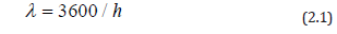
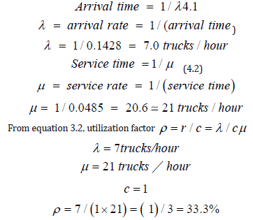
The input describes the way in which the customers arrive and join the system. Generally customers arrive neither in a more or less random fashion which is not worth making the prediction. Thus the arrival pattern can be described in terms of probabilities and consequently the probability distribution for inter arrival times (the time between two successive arrivals) must be defined. In other words the input is the rate at which customers arrive at a service facility. It is expressed in flow (customers/hr vehicles/hour in transportation scenario) or time headway (seconds/customer or seconds/vehicle in transportation scenario). If inter arrival time that is time headway (h) is known, the arrival rate can be found in Equation 2.1

The service mechanism (service pattern)

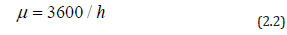
This means the arrangement facility to server customers. If there is infinite number of servers then all the customers are served instantly on arrival and there will be no queue. If the number of servers is finite then the customers are served according to a specific order with service time as a constant or a random variable. Distribution of service time which is important in practice is the negative exponential distribution. The mean service rate is denoted by μ. the service rate can be calculated from equation 2.2.

The queue discipline

Queue discipline is a parameter that explains how the customers arrive at a service facility.

The various types of queue disciplines are;

a. First in first out (FIFO)

b. First in last out (FILO)

c. Served in random order (SIRO)

d. Priority scheduling

e. Processor (or Time) Sharing

First in first out (FIFO)

If the customers are served in the order of their arrival, then this is known as the first-come, first-served (FCFS) service discipline. Prepaid taxi queue at airports where a taxi is engaged on a firstcome, first-served basis is an example of this discipline.

First in last out (FILO)

Sometimes, the customers are serviced in the reverse order of their entry so that the ones who join the last are served first. For example, assume that letters to be typed, or order forms to be processed accumulate in a pile, each new addition being put on the top of them. The typist or the clerk might process these letters or orders by taking each new task from the top of the pile. Thus, a just arriving task would be the next to be serviced provided that no fresh task arrives before it is picked up. Similarly, the people who join an elevator first are the last ones to leave it.

Served in random order (SIRO)

Under this rule, customers are selected for service randomly irrespective of their arrival in the service system. In this every customer in the queue is equally likely to be selected. The time of arrival of the customers is, therefore, of no relevance in such a case.

Priority service

Under this rule customers are grouped in priority classes on the basis of some attributes such as service time or urgency or according to some identifiable characteristic, and FIFO rule is used within each class to provide service. Treatment of VIPs in preference to other patients in a hospital is an example of priority service.

Processor (or time) sharing: the server is switched between all the queues for a predefined

Slice of time (quantum time) in a round-robin manner. Each queue head is served for that specific time. It doesn’t matter if the service is complete for a customer or not. If not then it’ll be served in its next turn. This is used to avoid the server time killed by customer for the external activities (e.g. preparing for payment or filling half-filled form).

Customer’s behavior

The customers generally behave in the following four ways:

Balking: The customer who leaves the queue because the queue is too long and he has no time to wait or has no sufficient waiting space.

Reneging: this occurs when a waiting customer leaves the queue due to impatience.

Priorities: In certain application some customers are served before the others regardless of their arrival. These customers have priority over others.

Jockeying: Customers may jockey from one waiting line to another.

System capacity

If a queue has a physical limitation to the number of customers that can be waiting in the system at one time, the maximum number of customers who can be receiving service and waiting is referred to as the system capacity. These are called finite queues since there is a finite limit to the maximum system size. If capacity is reached, no additional customers are allowed to enter the system.

Figure 2: Single channel queuing system [9].

The number of service stations in a queuing system refers to the number of servers operating in parallel that can service customers simultaneously. In a single channel service station, there is only one path that customers can take through the system. Figure 2 [9] shows the path customers, represented by circles; take through a single service channel queuing network. The customers arrive at the server, represented by the rectangle, and form a queue to wait for service if it is not immediately available, and then proceed through the system once service has been completed.

When there are multiple servers available operating in parallel, incoming customers can either wait for service by forming multiple queues at each server, as shown in (a) of Figure 3, or they can form a single queue where the first customer goes in line goes to the next available server, as shown in (b). Both of these types of queues are commonly found in day-to-day life. A single queue waiting for multiple servers is generally the preferred method, as it is more efficient at providing service to the incoming customers.

Figure 3: Multichannel queuing systems [9].

Notations

Queuing processes are frequently referred to by using a set of shorthand notation in the form of (a/b/c/): (d/e/f) where the symbols a through f stand for the characteristics shown in Table 1. The symbols a through f will take different abbreviations depending on what type of queuing symbols. A and b both represent types of distributions and may contain codes representing any of the common distributions listed in Table 2.

Table 1: Queuing notation abbreviations.

Table 2: Distribution abbreviations.

The spectrophotometric method [36] was used with slight modifications to determine mercury (II) concentrations in the samples. Dithiazone, in slightly acidic conditions, reacts with mercury (II) and produces an orange chelate (488nm absorption max). 10mg/ml of mercury (II) standard solution was prepared in a 100ml volumetric flask by dissolving 1.355g of mercuric chloride in distilled water. The stock solution was stored at 40 0C and used for all of the dilutions. A nine-point standard curve with concentrations ranging from 1 to 100μg/mL of mercury (II) was constructed, whereby 0.5ml of samples containing mercury (II) was combined with 0.5ml of dithiazone (37.2mg of dithiazone in 100ml of 1,4dioxane). Chelate was acidified with 0.05mL of 4.5M sulphuric acid, solubilized with 2.5mL of 1,4 dioxane and diluted with 1.45mL of distilled water to reach a total volume of 5.0 ml. A blank reagent with no mercury was prepared at the same time with 0.5mL of distilled water. Samples were incubated at room temperature (RT) for 24 hours and absorption at 488nm was determined against the blank using a Pharmacia Biotech Ultrospec 1000 (Cambridge, England) spectrophotometer with disposable acrylic cuvettes (BRAND GMBH+CO KG, Germany). The mercury concentrations of unknown samples were determined from the standard calibration curve (Figure 1).

Method of data analysis

In this research, the model adapted is the M/M/1: FCFS/∞/∞ queuing system. The model refers to negative exponential arrivals and service times with a single server and infinite queue length with an infinite population. This is the most widely used queuing systems in analysis and pretty much everything is known about it. M/M/1: FCFS/∞/∞ is a good approximation for a large number of queuing systems. Suitability of M/M/1: FCFS/∞/∞ queuing is easy to identify from the server standpoint. For instance a single transmit queue feeding a single link qualifies as a single server with an unlimited queue length and can be modeled as an M/M/1: FCFS/∞/∞ queuing system.

The model assumes a Poisson arrival process and exponentially distributed service process. This assumption is a very good approximation for arrival process in real systems that meet the following rules:

a) The number of customers in the system is very large.

b) The impact of a single customer for the performance of the system is very small, that is, a single customer consumes a very small percentage of the system resources.

c) All customers are independent, i.e. their decisions to use the system, does not depend on other users.

Model description

a) Arrivals are random, and come from the Poisson probability distribution (Markov input).

b) Each service time is also assumed to be a random variable following the exponential distribution (Markov service).

c) Service times are assumed to be independent of each other and independent of the arrival process.

d) There is one single server in the queue.

e) The queue discipline is First Come First Serve (FCFS) also known as first in first out, and there is no limit on the size of the line.

f) The average arrival and service rates do not change over time. The process has been operating long enough to remove effects of the initial conditions

Basic numeric characteristics of m/m/1: fcfs/∞/∞ queue

System must be operating long enough so that the probabilities resulting from the physical characteristics of the problem may satisfy the requirements of the mass selection of a statistical observation - that is, the system must be in equilibrium (steady state) .The characteristic of this queuing model can be classified as inputs and outputs.

Inputs

To use this model, the values for the number of loaders operating, the arrival rate of new trucks, and the service rate per loader must be known to be used as inputs to the model. The necessary inputs are outlined in the table below, The arrival rate, λ, is the average rate at which new trucks arrive at the loader. The service rate, μ, is the service rate of an individual loader. In cases with more than one loader in operation, all loaders are assumed to be equivalent, so μ would be the average service rate of the loaders. The arrival rate, λ, and service rate, μ, should both be input in the form of trucks per hour. Both the arrival rate and the service rate are independent of queue length.

Outputs

When given the appropriate inputs, the model calculates and outputs values for various aspects of pit activity. These include loader utilization; the average time a truck spends in the system, the average time a truck spends waiting to be loaded, the average number of trucks waiting in line, the average number of trucks in the system, and the system output in trucks per hour. Table 3 below lists the outputs created by the model and the appropriate units for each variable.

Table 3: Queuing model inputs.

Based on this queuing system and input variables, the variables r and ρ are defined as,

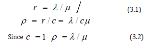
Where r is the expected number of trucks in service, or the offered workload rate, and ρ is defined as the traffic intensity or the service rate factor or loader utilization factor (Giffin, 1978). This is a measure of traffic congestion. When ρ > 1, or alternately λ >cμ where c is the number of loaders, the average number of truck arrivals into the system exceeds the maximum average service rate of the system and traffic will continue back up.

For situations when ρ > 1, the probability that there are zero trucks in the queuing system (Po) is defined as;

Where P0 = probability that there are zero trucks in the queuing system.

P₁ = Probability that there is one truck in the queuing system.

P₂ = Probability that there are two trucks in the queuing system.

P_n = Probability that there are n trucks in the queuing system.

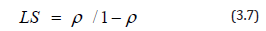
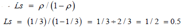
Where n is the number of trucks available in the haulage system. Even in situations with high loading rates, it is extremely likely that trucks will be delayed by waiting in line to be loaded. The queue length will have no definitive pattern when arrival and service rates are not deterministic, so the probability distribution of queue length is based on both the arrival rate and the loading rate [3]. The expected number of trucks in the system LS, can be calculated using the following equation.

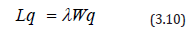
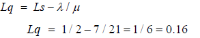
The expected number of trucks waiting to be loaded Lq, can be calculated using the formula below;

The average number of trucks in the queuing system, LS and the average time a truck spends waiting in line Wq can be found by applying Little’s formula which states that; the long term average number of customers in a stable system, LS, is equal to the long term average effective arrival rate, λ, multiplied by the average time a customer spends in the system, WS [3]. Little’s equation captures the relationship between the length of any system and time associated with the system. Mathematically, this is expressed as;

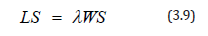
And can also be applied in the form

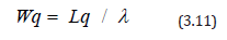
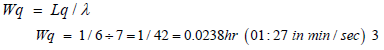
Using equations 3.10 & 3.11, the average time a truck spends waiting to be loadedWq can be calculated as follows.

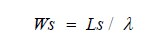
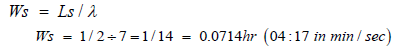
The average time a truck spends in the system, Ws, is defined as;

Presentation of inter-arrival time and service time

Table 4: Queuing model outputs.

From the (Table 4), the arrival times for five days at 2-4 hours per day were combined to form a list of all the trucks arrival for that shift. These arrival times were used to calculate the interarrival times of the trucks to be loaded. The inter-arrival time (time between each arrival) was calculated by taking the difference between each successive time of arriving trucks. Also, the time taken for the shovel to load trucks was also combined to form a list of the service time of all trucks for that shift.

Figure 4: Graph of frequency versusinter-arrival time.

Figure 5: Graph of frequency versus service time.

The inter-arrival times were fitted into the @risk software to create a graph of frequency versus time between new arrivals as shown in (Figure 4). Frequency is represented as a percentage of the total number of arrivals that occurs during the shift and arrival times in hours. The graph shows that the system follows an exponential manner which is an adequate fit for the inter-arrival times of trucks in the system. Also @risk software was able to compute the mean arrival time, standard deviation, minimum and maximum for both normal and exponential distribution as shown in the (Figure 5).

From (Figure 4) the minimum is 0.00330hr,the maximum is 0.8666hr,the mean arrival times is 0.1436hr and standard deviation is 0.1283 for a normal distribution while minimum is 0.00242hr,maximum is +∞,mean arrival time is 0.1428hr and standard deviation is 0.1403 for an exponential distribution.

The list of service times were fitted into the @risk software to create a graph of frequency versus service time with frequency represented in percentage of the total number of service rendered and service time represented in hour. (Figure 5) indicates that the service time follows an exponential distribution. The mean service time and standard deviation was automatically computed by @ risk software and it can be shown in the (Figure 5). The software computes minimum to be 0.0258.maximum to be 0.2358 mean service time to be 0.0486 and standard deviation to be 0.0225 for a normal distribution while minimum to be 0.0257,maximum to be +∞,mean service time to be 0.0485 and standard deviation to be 0.0228 for an exponential distribution.

Calculations of input and output characteristics of m/m/1: fcfs/∞/∞ model

From the graph, the mean arrival times is 0.1428hr and mean service time is 0.0485hr

From Equation 3.3, the probability that there are no trucks in the system, Po = 1-ρ

Probability that the serve is not free, that is there is a minimum of one truck in the system;

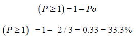
This means that 66.6% of the time, the server would be free and 33.3% of the time there would be at least one truck in the system.

Probability that there are no trucks queuing = Po + P1

From Equation 3.4, P1 = ρPo

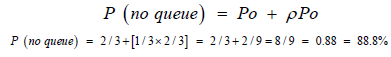
About 88.8% of the time, there will be no queue.

From Equation 3.7, the expected number of trucks in the system,

From Equation 3.8, the expected number of trucks in the system,

From Equation 3.12, the average waiting time in the system

From Equation 3.11, the average waiting time in the queue

Result of the input and output variables

The result from the calculation of the input and output are shown in the (Table 4).The queue will not have an impatient truck since it would be unrealistic for haul trucks not to join the line to be loaded regardless of how many trucks are already waiting. There would also be no jockeying for position since trucks form single line waiting to be served. The queuing model M/M/1: FCFS/∞/∞ is appropriate for this research because truck data from 12th to 16th October was examined and used to verify the queuing model created. This queuing model is useful for analysing the efficiency of mining haulage and loading operations for the configurations in which they are currently operating. The amount of time trucks spend waiting to be loaded, Wq, and the server utilization, ρ, are both indicators of how efficiently the system is operating. The larger the values of Wq, the longer trucks are spending idling waiting at the loaders, burning fuel without contributing to the haulage process. The server utilization indicates what proportion of operational time loaders are actually in use. Both of these values can be combined with costing data for the equipment in use to find out how much money is being spent on idling equipment.

Result shows that the arrival rate of the entire shift is 7 trucks per hour and service rate is 21 trucks per hour, this means that on an average, 7 trucks enters the system that is, every 8.59minsa truck arrives in the queue. And on average, 21 trucks are being served per hour meaning that every 2.86min, a truck leaves the system. Analysis also shows that the service rate is more than the arrival rate and this implies that there is going to be an increase in the idle probability. At every 66.6% of the time, the system is idle, in order to utilize the idle time, about 8 to 9 trucks can be added to the number of trucks entering every hour and by so doing the system has been duly optimized by maximizing the number of trucks entering per hour.

From (Table 5), the time trucks spent waiting to be loaded Wq is 1:27min/sec, with Wq having a smaller value, the waiting time is at a reduced level therefore, there is no problem of unnecessary burning of fuel while waiting. Also, the arrival and service rate were confirmed to fit exponential distributions. Optimization has been carried out by increasing the number of trucks entering per hour by 8 to 9trucks, and this will lead to an increase in productivity of the mine, efficient operation of the system and unnecessary cost in production process (Table 6).

Table 5: Result for inter-arrival time and service time between 12^th to 16^th of October, 2015.

Table 6: Result of the input and output variables.

Time of arrival at excavator area (hr/min/sec), time of first load by excavator into the truck (hr/min/sec), number of loads, time of departure from the excavator (hr/min/sec) and time taken to load trucks gotten from the Lafarge (sagamu plant) was analysed to develop a model M/M/1: FCFS/∞/∞, based on the assumption of single channel and single server with infinite number of queues. The model was used to calculate the arrival rate, service rate and number of server which at the end of it gives 7turcks/hour, 21trucks/hour and 1loader respectively. @risk software was used to fit both service and inter-arrival into exponential distribution. The result shows that as the size of the haulage truck being used increases, shovel productivity increases and truck productivity decreases. An effective number of trucks must be chosen that will effectively utilize idle time, increase productivity and reduce cost of production to the barest minimum. The result shows 66.6% idle time; this indicates that an additional 8 to 9 trucks can be added to the company truck fleet to make use of the idle time; since time translate to cost.

1. Ercelebi SG, Bascetin A (2009) Optimization of shovel-truck system for surfacemining. The Journal of the Southern African Institute of Mining and Metallurgy 109(7): 433-439.
2. Najor J, Hagan P (2004) Mine Production Scheduling within Capacity Constraints. The University of New South Wales Sydney, Australia, p. 102.
3. Gross D, Harris CM (1998) Fundamentals of queuing theory. In: John Wiley & Sons, (4th edn), New York, USA, p. 528.
4. Munisamy S, Balakhrishnam B (2007) Performancy analysis and stall planning in a telecommunications contact centre - a queuing theory approach. International Review of Business Research Papers 3(3): 219- 241.
5. Odior AO (2013) Application of queuing theory to petrol stations in benincity area of edo state, Nigeria. Nigerian Journal of Technology 32(2): 325-332.
6. Anokye M, Abdul Aziz AR, Annin K, Oduro FT (2013) Application of queuing theory to vehicular traffic at signalized intersection in Kumasi- Ashanti Region, Ghana. American International Journal of Contemporary Research 3(7): 23-29.
7. Ghimire S, Thapa GB, Ghimire RP, Silvestov S (2017) A survey on queuing systems with mathematical models and application. American Journal of Operation Research 7(1): 1-14.
8. Soubhagya S (2012) Truck allocation model using linear programming and queuing theory, pp. 1-20.
9. May AM (2012) Application of queuing theory for open-pit truck/shovel haulage system. Master’s ScienceInMining & Minerals Engineering, Virginia Polytechnic Institute and State University, p. 72.